6.2 LINES/CURVES
Lines and curves are typically fit to data points.
A spline based curve is typically represented with a polynomial.
6.2.1 Lines
Lines are typically represented in a parametric form. As we vary a parameter we move along the line. (Note: typical parameter variables are s,t,u,v)

Note: lines can also be represented in explicit form, although this is not as useful for mathematical modeling.

6.2.2 Splines
A spline curve can interpolate or approximate a curve,

A bumpy curve will require a more complicated function (a polynomial with more degrees of freedom).
6.2.2.1 - Cubic
A cubic spline typically gives the best data fit. The example below is a parametric fit to four data points.
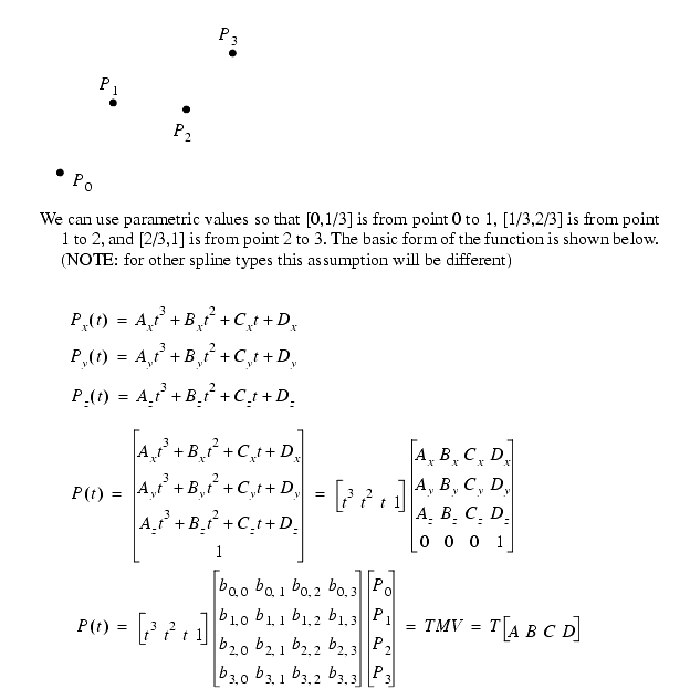
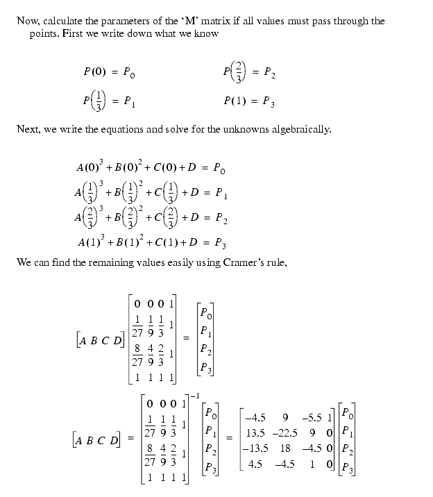
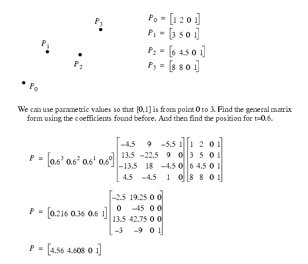
As we deal with different splines, the coefficient matrix changes,
some of the different spline types are,
6.2.2.2 - Bezier Curves
A bezier curve is approximated. The two endpoints are clearly defined, but the two inside points determine the internal shape by setting slopes at the ends,

Consider the shape of these curves are fixed to go through the endpoints, but are only guided by the two internal points
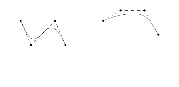
Instead of the matrix form for representing splines, we can also use blending functions (the results are the same for a 4 point set). And, this allows us to generalize to a larger number of degrees of freedom.

When using blending functions we can easily use more than three points (n=3) to define the spline.
Bezier curves are distinctive in that changing an endpoint or control point will change the shape of the entire curve.
6.2.2.3 - Ferguson/Hermite Curves
These curves are defined by endpoints and slopes at the endpoints. Note - here we need to specify derivatives.

These curves are of the greatest use when the endpoints of the line, and the slopes at those points are of more interest than the internal shape of the curve.
6.2.2.4 - Catmull-Rom Curves
These curves go through every point, but we have a tightness variable `c'.
As the value of `c' goes to zero, the connecting lines become straight.
The basic form of the matrix is,

6.2.2.5 - B-Splines
***************** REVISE TO CLARIFY **************************
B-Splines are typically defined using blending functions, and they will often have more than four points in their definition.
The basic form for the nonuniform B-Spline is shown below in the Cox-deBoor recursive function.
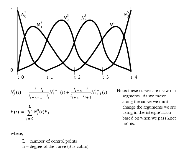
If the intervals are all equal we call this uniform. When the intervals are different lengths we call this nonuniform. A nonuniform curve can take on much more complicated shapes.

We can also weight the points to increase their effects on the final curve shape. This creates a rational spline.

Non-Rational Uniform B-Spline (NURBS) curves are popular in CAD systems as they are the most general form of the spline curves. They combine both the rational weighting of points, and non-uniform knot spacing.
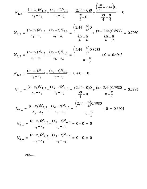
Find a point at 140 degrees for NURB curve that models a sine wave from 0 to 180 degrees.

6.2.3 Advanced Splines
We can sometimes double up (or more) points to increase the effect of a weighting. This is more valuable when the function is not rational. If we do this in the middle of a curve it tends to pull the curve tight. When done at the ends it makes the ends more regular.

Quite often we will attach two spline segments in series. The connection between the segments will be said to have continuity. A zero order continuity means they touch, 1st order means they are smooth, etc. It is easier to ensure continuity with splines such as the Ferguson.
A closed spline curve fully connects back to itself. (i.e., forms a loop)