13.2 MOTION PROFILES
������������
13.2.1 Velocity Profiles
������������
A simple example of a velocity profile for a point-to-point motion is shown in Figure 1.77. In this example the motion starts at 20 deg and ends at 100 deg. (Note: in motion controllers it is more common to used encoder pulses, instead of degrees, for positions velocities, etc.) For position control we want a motion that has a velocity of zero at the start and end of the motion, and accelerates and decelerates smoothly.
Figure 1.77 An example of a desired motion (position)
A trapezoidal velocity profile is shown in Figure 1.78. The area under the curve is the total distance moved. The slope of the initial and final ramp are the maximum acceleration and deceleration. The top level of the trapezoid is the maximum velocity. Some controllers allow the user to use the acceleration and deceleration times instead of the maximum acceleration and deceleration. This profile gives a continuous acceleration, but there will be a jerk (third order derivative) at the four sharp corners.
Figure 1.78 An example of a velocity profile
The basic relationships for these variables are shown in Figure 1.79. The equations can be used to find the acceleration and deceleration times. These equations can also be used to find the time at the maximum velocity. If this time is negative it indicates that the axis will not reach the maximum velocity, and the acceleration and deceleration times must be decreased. The resulting velocity profile will be a triangle.
Figure 1.79 Velocity profile basic relationships
For the example in Figure 1.80 the move starts at 100deg and ends at 20 deg. The acceleration and decelerations are completed in half a second. The system moves for 7.5 seconds at the maximum velocity.
Figure 1.80 Velocity profile example
The motion example in Figure 1.81 is so short the axis never reaches the maximum velocity. This is made obvious by the negative time at maximum velocity. In place of this the acceleration and deceleration times can be calculated by using the basic acceleration position relationship. The result in this example is a motion that accelerates for 0.316s and then decelerates for the same time.
Figure 1.81 Velocity profile example without reaching maximum velocity
Given the parameters calculated for the motion, the setpoints for motion can be calculated with the equations in Figure 1.82.
Figure 1.82 Generating points given motion parameters
A subroutine that implements these is shown in Figure 1.83. In this subroutine the time is looped with fixed time steps. The position setpoint values are put into the setpoint array, which will then be used elsewhere to guide the mechanism.
Figure 1.83 Subroutine for calculating motion setpoints
In some cases the jerk should be minimized. This can be achieved by replacing the acceleration ramps with a smooth polynomial, as shown in Figure 1.84. In this case two quadratic polynomials will be used for the acceleration, and another two for the deceleration.
Figure 1.84 A smooth velocity profile
An example of calculating the polynomial coefficients is given in Figure 1.85. The curve found is for the first half of the acceleration. It can then be used for the three other required curves.
Figure 1.85 A smooth velocity profile example
Figure 1.86 A smooth velocity profile example (cont'd)
13.2.2 Position Profiles
������������
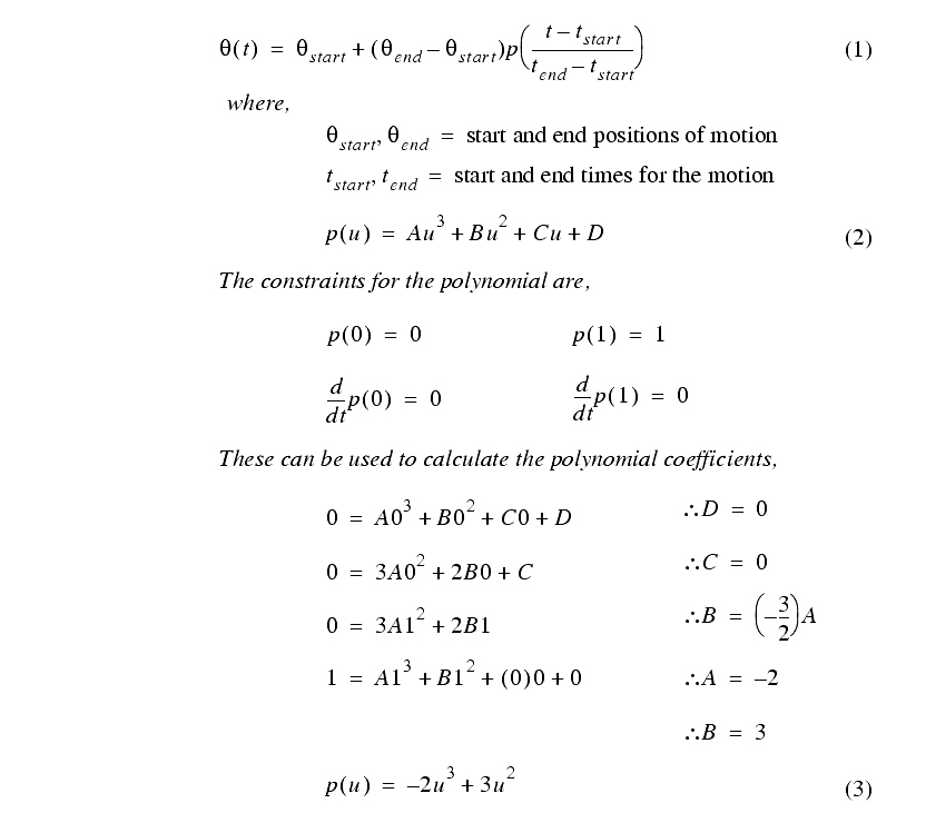
A motion can be described using position points along a path. These methods are normally used when a controller does not have any velocity or acceleration limits. The method shown in Figure 1.87 controls motion using a parametric function 'p(u)'. The function value varies from 0 to 1 as the parameter 'u' varies from 0 to 1. However, the parameters of the function are selected so that the motion starts and stops with a velocity of zero. In this case the final polynomial equation, (3), is fairly simple. This equation can then be used in equation (1) to generate a smooth motion path between any arbitrary start and end point, with arbitrary start and end times.
Figure 1.87 Generating smooth motion paths
The example in Figure 1.88 shows the use of a trigonometric function, instead of a polynomial. This function was used to generate the points in the following sample program in Figure 1.89.
Figure 1.88 Generating smooth motion paths
The program in Figure 1.89 generates a motion table that can then be used to update setpoints. The function 'table_init()' must be called once when the program starts to set up global time and table values. When a new target position has been specified the 'table_generate()' function is called to generate the setpoint table. The 'table_update()' function is called once every interrupt scan to check the setpoint table, and update the global setpoint variable, 'point_current' at scheduled times. This function also includes a simple clock to keep track of the system time.
Figure 1.89 Subroutines for motion profile generation and use


