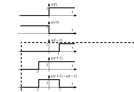
When analyzing a system, we may need to choose an input that is more complex than inputs such as steps, ramps, sinusoids and parabolae. The easiest way to do this is to use switching functions. Switching functions turn on (have a value of 1) when their arguments are greater than or equal to zero, or off (a value of 0) when the argument is negative. Examples of the use of switching functions are shown in Figure 4.33 Example: Switching functions. By changing the values of the arguments we can change when a function turns on or off.

Figure 4.33 Example: Switching functions
These switching functions can be multiplied with other functions to create a complex function by turning parts of the function on or off. An example of a curve created with switching functions is shown in Figure 4.34 Example: Switching functions to create a non-smooth function.
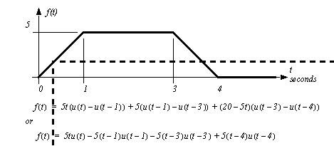
Figure 4.34 Example: Switching functions to create a non-smooth function
The unit step switching function is available in Mathcad and makes creation of complex functions relatively trivial. Step functions are also easy to implement when writing computer programs, as shown in Figure 4.35 Example: A subroutine implementing the example in Figure 4.34.

Figure 4.35 Example: A subroutine implementing the example in Figure 4.34 Example: Switching functions to create a non-smooth function
In some cases we are given tables of numbers instead of equations for a system component. These can still be used to do numerical integration by calculating coefficient values as required, in place of an equation.
Tabular data consists of separate data points as seen in Figure 4.36 Example: Using tables of values to interpolate numerical values using the lever law. But, we may need values between the datapoints. A simple method for finding intermediate values is to interpolate with the "lever law". (Note: it is called this because of its’ similarity to the equation for a lever.) The table in the example only gives flow rates for a valve at 10 degree intervals, but we want flow rates at 46 and 23 degrees. A simple application of the lever law gives approximate values for the flow rates.
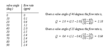
Figure 4.36 Example: Using tables of values to interpolate numerical values using the lever law
The subroutine in Figure 4.37 Example: A tabular interpolation subroutine was written to return the numerical value for the data table in Figure 4.36 Example: Using tables of values to interpolate numerical values using the lever law. In the subroutine the tabular data is examined to find the interval that the flow rate value falls inside. Once this is found the valve angle is calculated as the ratio between the two known values.
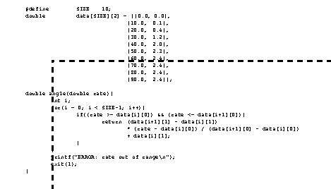
Figure 4.37 Example: A tabular interpolation subroutine
When greater accuracy is required, smooth curves can be fitted to interpolate points. These curves are known as splines. There are multiple methods for creating splines, but the simplest is to use a polynomial fitted to a set of points.
The example in Figure 4.38 Example: Spline fitting shows a spline curve being fitted for three data points. In this case a second order polynomial is used. The three data points are written out as equations, and then put into matrix form, using the coefficients as the unknown values. The matrix is then solved to obtain the coefficient values for the final equation. This equation can then be used to build a mathematical model of the system.
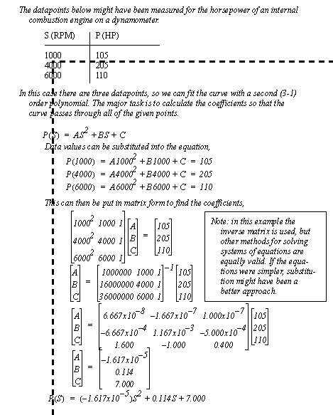
Figure 4.38 Example: Spline fitting
The order of the polynomial should match the number of points. Although, as the number of points increases, the shape of the curve will become less smooth. A common way for dealing with this problem is to fit the spline to a smaller number of points and then verify that it matches the remaining points, or use a least squares method to find the best approximation.
Despite our deepest wishes for simplicity, most systems contain non-linear components. In the last chapter we looked at dealing with non-linearities by linearizing them locally. Numerical techniques will handle non-linearities easily, but smaller time steps are required for accuracy.
Consider the mass and an applied force shown in Figure 4.39 Example: Developing state equations for a non-linear system. As the mass moves an aerodynamic resistance force is generated that is proportional to the square of the velocity. This results in a non-linear differential equation. This equation can be numerically integrated using a technique such as Runge-Kutta. Note that the state equation matrix form cannot be used because it requires linear equations.

Figure 4.39 Example: Developing state equations for a non-linear system