The general process of analyzing systems of differential equations involves first putting the equations into standard form, and then integrating these with one of a number of techniques. State variable equations are the most common standard equation form. In this form all of the equations are reduced to first-order differential equations. These first-order equations are then easily integrated to provide a solution for the system of equations.
At any time a system can be said to have a state. Consider a car for example, the state of the car is described by its position and velocity. Factors that are useful when identifying state variables are:
• The variables should describe energy storing elements (potential or kinetic).
• The variables must be independent.
• They should fully describe the system elements.
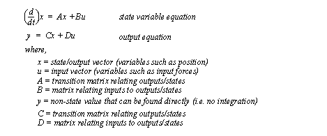
After the state variables of a system have been identified, they can be used to write first-order state variable equations. The general form of state variable equations is shown in Figure 4.1 The general state variable form. Notice that the state variable equation is linear, and the value of x is used to calculate the derivative. The output equation is not always required, but it can be used to calculate new output values.

Figure 4.1 The general state variable form
An example of a state variable equation is shown in Figure 4.2 Example: A state variable equation. As always, the FBD is used to develop the differential equation. The resulting differential equation is second-order, but this must be reduced to first-order. Using the velocity variable, ’v’ the second-order differential equation can be reduced to a first-order equation. An equation is also required to define the velocity as the first derivative of the position, ’x’. In the example the two state equations are manipulated into a matrix form. This form can be useful, and may be required for determining a solution. For example, HP calculators require the matrix form, while TI calculators use the equation forms. Software such as Mathcad can use either form. The main disadvantage of the matrix form is that it will only work for linear differential equations.
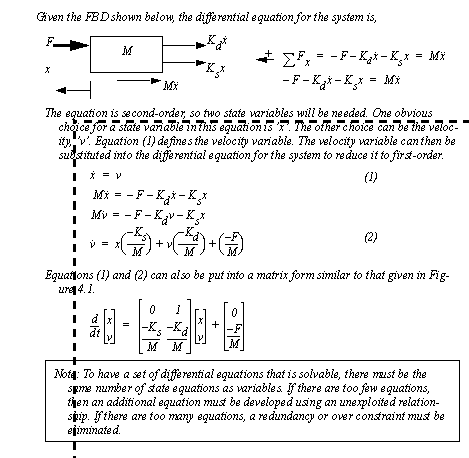
Figure 4.2 Example: A state variable equation
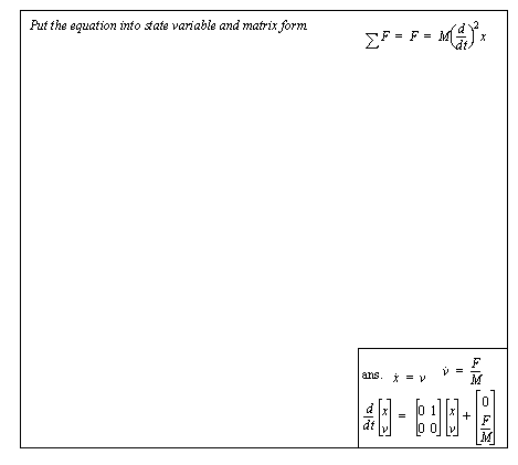
Figure 4.3 Drill problem: Put the equation in state variable form
Consider the two cart problem in Figure 4.4 Example: Two cart state equation. The carts are separated from each other and the wall by springs, and a force is applied to the left hand side. Free body diagrams are developed for each of the carts, and differential equations developed. For each cart a velocity state variable is created. The equations are then manipulated to convert the second-order differential equations to first-order state equations. The four resulting equations are then put into the state variable matrix form.
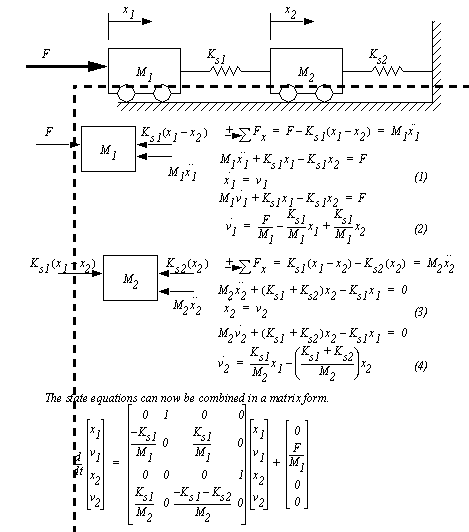
Figure 4.4 Example: Two cart state equation
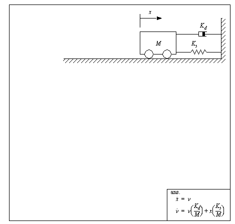
Figure 4.5 Drill problem: Develop the state equations in matrix form
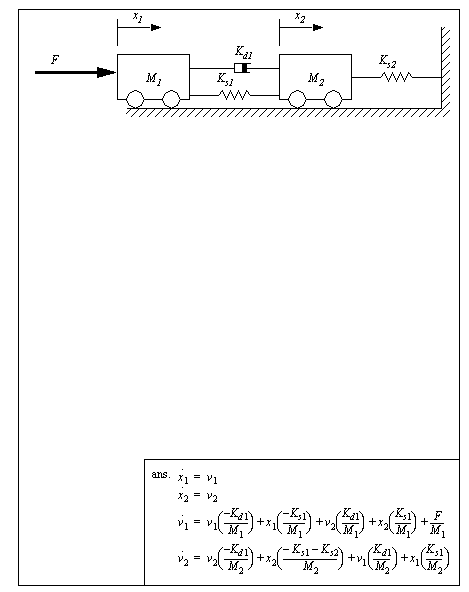
Figure 4.6 Drill problem: Convert the system to state equations
In some cases we will develop differential equations that cannot be directly reduced because they have more than one term at the highest order. For example, if a second-order differential equation has two second derivatives it cannot be converted to a state equation in the normal manner. In this case the two high order derivatives can be replaced with a dummy variable. In mechanical systems this often happens when masses are neglected. Consider the example problem in Figure 4.7 Using dummy variables for multiple high order terms, both ’y’ and ’u’ are first derivatives. To solve this problem, the highest order terms (’y’ and ’u’) are moved to the left of the equation. A dummy variable, ’q’, is then created to replace these two variables with a single variable. This also creates an output equation as shown in Figure 4.1 The general state variable form.
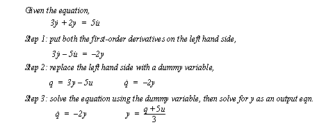
Figure 4.7 Using dummy variables for multiple high order terms
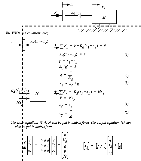
At other times it is possible to eliminate redundant terms through algebraic manipulation, as shown in Figure 4.8 Example: A dummy variable. In this case the force on both sides of the damper is the same, so it is substituted into the equation for the cart. But, the effects on the damper must also be integrated, so a dummy variable is created for the integration. An output equation was created to calculate the value for x 1 .
