1.6.1 Selection of Machining Processes

Machining is distinguished by the successive removal of material. The order of removal, the tools and fixtures chosen, and other factors all have a profound impact on the cost. As discussed before, a good mix of AI and algorithms will result in a more successful system, and this will be obvious throughout this section.

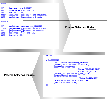
1.6.2 Selection of Machine Tools

There are many ways to choose machining details such as: tools, coolants, fixtures, etc. Methods for selecting include rules, frames, etc. (see Figure 1.10 Rules and Frames for Machine Selection).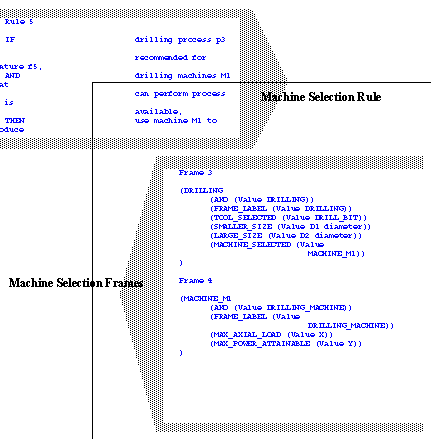

 

Figure 1.10 Rules and Frames for Machine Selection

(Adapted from [Kusiak, 1991])

1.6.3 Machining Optimization

The very nature of manufacturing is such that a manufacturer must survive through outperforming the competition. To do this there are a number of objectives the manufacturer will try to meet through optimizing some aspects of production. These objectives vary, and alter how decisions are made within the factory. Process planning has a large effect on the cost of production. By considering optimization of processes during the planning there can be considerable savings.

The machining optimization problem has some fundamental elements found in all optimization problems. Cost tends to rule all decisions. This results from a number of interrelated factors,

• tool life,

• machining time,

• tool cost,

• etc.

Each of these can be estimated using approximations. For example, tool wear may be estimated using Taylor’s tool life equation,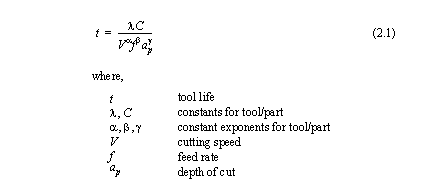

Machining time is greatly affected by the number of passes. The single pass model is fairly simple, and can be formulated as a constrained optimization problem. The multi-pass model is similar, but has added parameters to account for the multiple passes. Kusiak [1991] discusses the model shown in Figure 1.11 Parameters of the Multi-pass Machining Model. Please note that the single-pass model is ignored because it may be easily derived from the multi-pass model.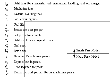

 

Figure 1.11 Parameters of the Multi-pass Machining Model

(Adapted from Kusiak [1991, pp. 261-262])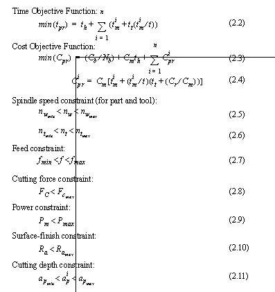

 

Figure 1.12 Objective and Constraints of Multi-pass Machining Model

There are many approaches used for optimization. Challa and Berra[1976] used a gradient search method. Chang et. al. [1982] used dynamic programming, after putting some variables in the discrete domain. Kusiak [1987] presents a hybrid system for knowledge based, and numerical optimization of the problem.

 

1.6.4 Optimal Selection of Machinable Volumes

A large machinable volume will require multiple passes of a tool. To determine the sub-volumes, it should be decomposed using some geometrical methods. The example in Figure 1.13 Decomposition of a Machinable Volume shows how a part has been decomposed by extending the planes describing the surfaces.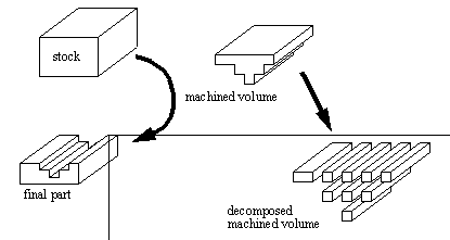

 

Figure 1.13 Decomposition of a Machinable Volume

This decomposition is easily accomplished if the planes existing in the part, are extended, and used as cutting planes, for the machined volume.

When a machinable volume has been decomposed, each of the volumes may be further sub-divided into elemental volumes. The fully decomposed volume is shown in Figure 1.14 A Machinable Volume Sub-Divided into Elementary Volumes.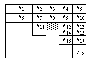

 

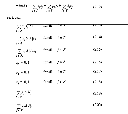
Figure 1.14 A Machinable Volume Sub-Divided into Elementary Volumes

(Adapted from [Kusiak, 1991])

After dividing the machinable volume, the problem may be approached as an optimization problem. The list of variables in Figure 1.15 Decision Variables for Optimal Machinable Volume Selection defines the decision variables involved with the problem. The Objective function, and the constraints are shown in Figure 1.16 Objective and Constraints for Selection of Machinable Volumes. This formulation is taken from Kusiak [1991]. He states that this formulation should be complete. He also states that some of the constraints and variables may be ignored in some problems.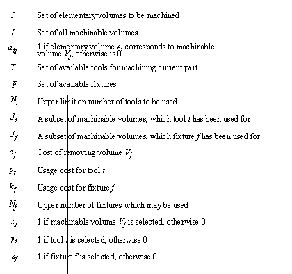

 

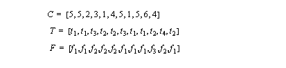
Figure 1.15 Decision Variables for Optimal Machinable Volume Selection

(Adapted from [Kusiak, 1991])

 

 

Figure 1.16 Objective and Constraints for Selection of Machinable Volumes

(Adapted from [Kusiak, 1991])

The example in Kusiak [1991] goes on to show a machinable volume matrix, shown here in Figure 1.17 A Machinable Volume Matrix. The matrix shows that there are a number of possible ways to machine the volumes (not all must be used). These volumes also correspond to costs, tools, and fixtures (shown in Figure 1.18 Example Sets for Machinable Volume Matrix). These also generate a precedence graph (shown in Figure 1.20 Precedence Graph and Rules for Machinable Volumes).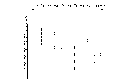

 

Figure 1.17 A Machinable Volume Matrix

(Adapted from [Kusiak, 1991])

 

Figure 1.18 Example Sets for Machinable Volume Matrix

In addition to this, the constraints that Nt = 3, and Nf = 2 are added for this example. The resulting solution is developed using unspecified optimization techniques, and is shown below in Figure 1.19 Solution for Example Problem.

 

Figure 1.19 Solution for Example Problem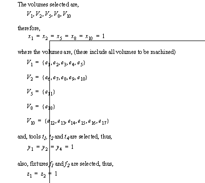

The solution produces an objective function value of Z = 23. Kusiak claims that this solution reduces cutting costs by as much as 8%, and reduces the tool and fixture count over traditional methods.

To continue this example, consider that the sequence of operations is not yet determined. This may be done using simple rules about volume relations. The relations are mainly based on i) accessibility of volume, and ii) datums for tolerances. Some examples of rules are given by Kusiak [1991], and shown here in Figure 1.20 Precedence Graph and Rules for Machinable Volumes.

 

Figure 1.20 Precedence Graph and Rules for Machinable Volumes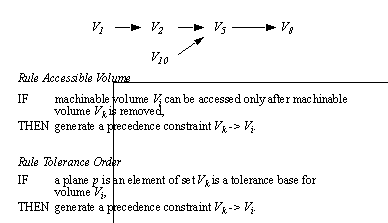

(to Produce the Precedence Relations)

After the precedence constraints have been determined, the operations must be sequenced. This is done by first checking to see that there are some start nodes, with no predecessors, to ensure that the precedence graph is solvable. If it is then starting from the left the graph is expanded. The two possible sequences are {V1, V2, V10, V5, V8}, and {V1, V10, V2, V5, V8}. In his paper, Kusiak [1991] does not suggest how to resolve this dilemma, but does mention setup costs are one possible method.

The work of Kusiak is of importance to this thesis when considering what BCAPP must do. By itself Kusiak’s work describes a complete operation planner for some forms of machining. But, without first selecting machining, and then specifying features to machined, it has reduced value. Therefore, after the process plan is completed by BCAPP, a system like the one described here should be used to select tools, cuts, speeds, feeds, etc.