STRAIGHT LINE APPROXIMATIONSAn approximate technique for constructing a gain Bode plot is shown in Figure 10.10 The method for Bode graph straight line gain approximation. This method involves looking at the transfer function and reducing it to roots in the numerator and denominator. Once in that form, a straight line approximation for each term can be drawn on the graph. An initial gain is also calculated to shift the results up or down. When done, the straight line segments are added to produce a more complex straight line curve. A smooth curve is then drawn over top of this curve. 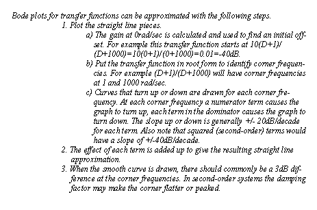
Figure 10.10 The method for Bode graph straight line gain approximation 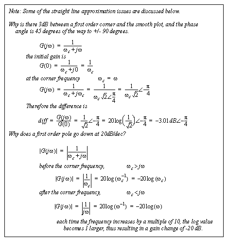
Figure 10.11 Why the straight line method works 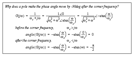
Figure 10.12 Why the straight line method works (cont’d) 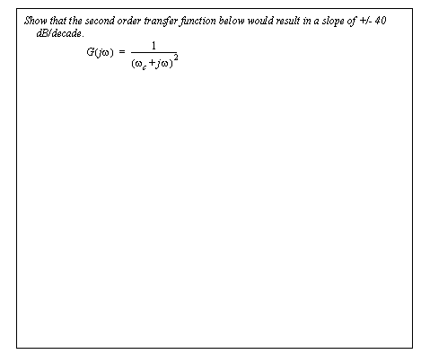
Figure 10.13 Drill problem: Slope of second order transfer functions. An example of the straight line plotting technique is shown in Figure 10.14 An approximate gain plot example. In this example the transfer function is first put into a root form. In total there are three roots, 1, 10 and 100 rad/sec. The single root in the numerator will cause the curve to start upward with a slope of 20dB/dec after 1rad/sec. The two roots will cause two curves downwards at -20dB/dec starting at 10 and 100 rad/sec. The initial gain of the transfer function is also calculated, and converted to decibels. The frequency axis is rad/sec by default, but if Hz are used then it is necessary to convert the values. 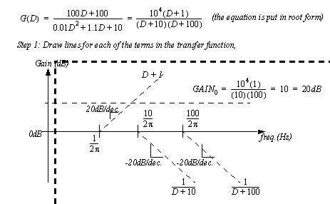
Figure 10.14 An approximate gain plot example The example is continued in Figure 10.15 An approximate gain plot example (continued) where the straight line segments are added to produce a combined straight line curve. 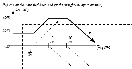
Figure 10.15 An approximate gain plot example (continued) Finally a smooth curve is fitted to the straight line approximation. When drawing the curve imagine that there are rubber bands at the corners that pull slightly and smooth out. For a simple first-order term there is a 3dB gap between the sharp corner and the function. Higher order functions will be discussed later. 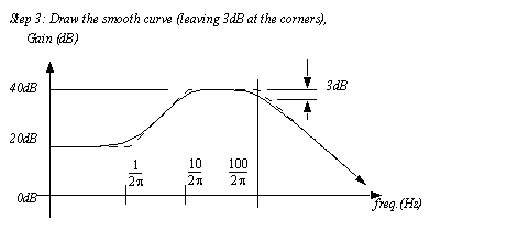
Figure 10.16 An approximate gain plot example (continued) The process for constructing phase plots is similar to that of gain plots, as seen in Figure 10.18 An approximate phase plot example. The transfer function is put into root form, and then straight line phase shifts are drawn for each of the terms. Each term in the numerator will cause a positive shift of 90 degrees, while terms in the denominator cause negative shifts of 90 degrees. The phase shift occurs over two decades, meaning that for a center frequency of 100, the shift would start at 10 and end at 1000. If there are any lone ’D’ terms on the top or bottom, they will each shift the initial value by 90 degrees, otherwise the phase should start at 0degrees. 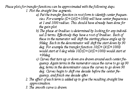
Figure 10.17 The method for Bode graph straight line gain approximation The previous example started in Figure 10.14 An approximate gain plot example is continued in Figure 10.18 An approximate phase plot example to develop a phase plot using the approximate technique. There are three roots for the transfer function. None of these are zero, so the phase plot starts at zero degrees. The root in the numerator causes a shift of positive 90 deg, starting one decade before 1rad/sec and ending one decade later. The two roots in the denominator cause a shift downward. 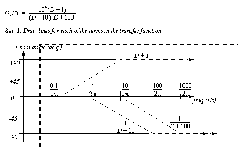
Figure 10.18 An approximate phase plot example The straight line segments for the phase plot are added in Figure 10.19 An approximate phase plot example (continued) to produce a straight line approximation of the final plot. A smooth line approximation is drawn using the straight line as a guide. Again, the concept of a rubber band will smooth the curve. 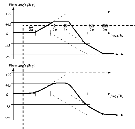
Figure 10.19 An approximate phase plot example (continued) 10.3.1 Second Order Underdamped TermsThe previous example used a transfer function with real roots. In a second-order system with double real roots (overdamped) the curve can be drawn with two overlapping straight line approximations. If the roots for the transfer function are complex (underdamped the corner frequencies will become peaked. This can be handled by determining the damping factor and natural frequency as shown in Figure 10.20 Resonant peaks. The peak will occur at the damped frequency. The peaking effect will become more pronounced as the damping factor goes from 0.707 to 0 where the peak will be infinite. 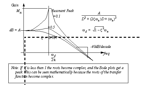
The approximate techniques do decrease the accuracy of the final solution, but they can be calculated quickly. In addition these curves provide an understanding of the system that makes design easier. For example, a designer will often describe a system with a Bode plot, and then convert this to a desired transfer function. 
Figure 10.21 Drill problem: Draw the straight line approximation 10.3.2 Lone Ds on the Top or BottomIn some cases the transfer function will have a lone ’D’ on the top or bottom. In these cases it means that the gain of the system starts (i.e., f = 0Hz) starts at infinity for a ’D’ on the bottom, or at a gain of 0 (negative infinity dB) for a ’D’ on the top.Or in other words, consider the Ds to have corner frequencies at zero. This means that Ds on the top start at infinity and come down. Ds on the bottom start at negative infinity and come up. If at all possible cancel the Ds on the top and bottom, if any remain then to draw the Bode plot you must work from the right side of the graph (i.e. f = infinity Hz). Consider the example in Figure 10.22 A System Gain Starting at Negative Infinity. The D squared term on the top is squared, so the system is second order and the phase angle starts at 180 degrees. The gain starts at 0 (-infinity dB) goes upwards at 40dB/dec. As the upward slope of +40dB/dec approaches the corner frequency of the bottom, with a slope of -40dB/dec, the two effects cancel and the slope becomes 0, for a vertical line. The problem solution is similar when the lone Ds are on the bottom. With these types of problems the top and bottom of the transfer function might go to zero or infinity. Normally we would say this is underdefined. In these cases, L’Hospital’s rule may be used. 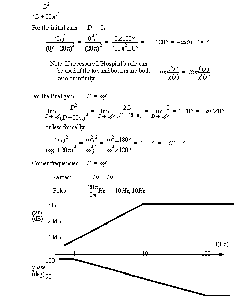
Figure 10.22 A System Gain Starting at Negative Infinity In all of the examples presented, were we start or stop could be drawn from the left or right. This will not always be the case as shown in the Figure 10.23 Calculating a point to set a position. In this case the term on the top results in a slope of +20dB/dec on the left. The order of the numerator and denominator are not the same so the final result will not be horizontal. The bottom is second order, compared to the first order top, so the final result will be a downward slope of -20dB/dec. This leaves the dilema of where the graph starts and ends. The solution is to calculate one or more points on the curve using phasor transforms. 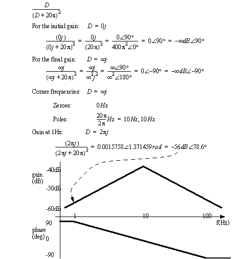
|