PRACTICAL ELEMENTS OF COMPUTER MATHAs engineers we use computers to perform many calculation quickly. There is an obvious trade-off between computer cost and speed. And, of course, more precision is more costly. For example, if we are using a desktop system for the analysis of experimental data we may be able to buy an expensive computer with a high level of mathematical precision. However a microprocessor that is to be put into an automotive part must have a very low cost. Many computers have math functions built into an Arithmatic Logic Unit (ALU) core. On smaller microcontrollers this will often do integer (2s compliment) addition, subtraction, multiplication, and division. More advanced computers will include a mathematic co-processor unit that is dedicated to returning floating point numerical results quickly. 4.7.1 Numbering SystemsComputer based number representations are ultimately reduced to true or false values. The simplest number is a binary bit with an integer range from 0 to 1, however bits are normally grouped into some larger multiple of 8 based upon the size of the date bus (e.g., 8-byte, 16-word, 32- long word, 64). These are then used to represent numerical values over a range. For example a byte can respresent an unsigned integer value from 0 to 255, a signed integer value from -127 to 127, or a 2s compliment integer value from -128 to 127. As expected the precision and range of the number increases with the number of bits. And, by allocating a few of the bits for an exponent, the number can be used to represent large real values. Figure 4.40 Typical Number System Tradeoffs shows a very simplistic comparison of the number systems. 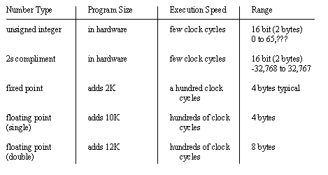
Figure 4.40 Typical Number System Tradeoffs The subject of computer numbering systems is very broad and this book is not intended to teach the fundamentals of these numbering systems. But, to provide some design direction, • If possible use 2s compliment integer calculations with 2 or 4 bytes. These will run easily on inexpensive hardware, And if used on faster computers there will be a substantial speed bonus. The problems are the limited range and loss of fractions. • Floating point calculations are the standard on regular (non-embedded) computers. The numbers are 7 place, single precision, 4 byte numbers or 14 place, double precision, 8 byte numbers. Unless space is at a premium, use double precision. To implement these subroutines in small computers can consume large amounts of available memory and processor time. • Fixed point numbers do not allow all of the flexibility of the floating point values, but preserve the fractional results. These are often used to get the speed or memory benefits of floating point calculations on lower end computers. Figure 4.41 Example: Program speed based upon number system shows two subroutines that are effectively identical, except for the choice of number system. Both will loop 999 times, incrementing the index value by adding one. The print statement within the loop also requires are division and modulo operations. All three of the mathematical operations are slower for double precision. Moreover the printf statement will require more time to print the results for the floating point numbers. Overall the integer loop will probably run an order of magnitude faster. 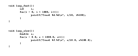
Figure 4.41 Example: Program speed based upon number system 4.7.2 SpeedIn the design of controls systems the execution time for a program may be critical to system stability. Or, when running large numerical calculations, small changes can save days or weeks of computer time. Each operation requires a finite number of computer CPU cycles with the number varying based upon the instruction. For example a sign change is very fast, addition and subtraction can be slower, multiplication and division slower still, and a trigonometric operation is among the slowest. If the operations are done in hardware they will be much faster. If done in software the speed will vary depending upon the compiler. It is often possible to reduce the computation time by reducing the number of slower operations. In Figure 4.42 Rearranging Expressions to Increase Execution Speed there is a simple manipulation that eliminates one addition, or a more elaborate method that eliminates one trigonometric operation. In practice this would probably reduce the calculation time by at least one quarter to a half. 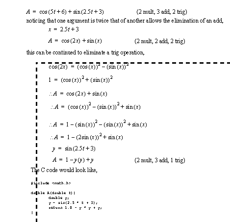
Figure 4.42 Rearranging Expressions to Increase Execution Speed 4.7.3 AccuracyComputer calculations are generally repeatable - meaning that repeating a calculation will give exactly the same result. Although this does not mean that the result is correct. For example a small error (one in a million) repeated a million times becomes significant. Considering the iterative nature of numerical calculations this scenario is likely to occur (note: not just possible). In these cases it is important to review the results with the following rules. • Understand that the magnitude of errors increases with the number of calculations. • Find a way to measure errors in calculations. • Where possible correct for errors in calculations. A common problem with floating point numbers is determining when the values are equal. Consider the values 2.00000001 and 1.99999998, for all practical purposes they are equal. But, from the standpoint of a computer they differ by 0.00000003 and are not equal. This can be overcome using a subroutine like that shown in Figure 4.43 Example: Error Allowances for Equivalences. 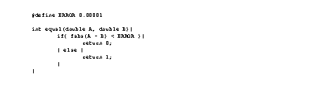
|