NUMERICAL INTEGRATION

Repetitive calculations can be used to develop an approximate solution to a set of differential equations. Starting from given initial conditions, the equation is solved with small time steps. Smaller time steps result in a higher level of accuracy, while larger time steps give a faster solution.

Numerical solutions can be developed with hand calculations, but this is a very time consuming task. In this section we will explore some common tools for solving state variable equations. The analysis process follows the basic steps listed below.

1. Generate the differential equations to model the process.

2. Select the state variables.

3. Rearrange the equations to state variable form.

4. Add additional equations as required.

5. Enter the equations into a computer or calculator and solve.

An example in Figure 4.9 Example: Dynamic system shows the first four steps for a mass-spring-damper combination. The FBD is used to develop the differential equations for the system. The state variables are then selected, in this case the position, y, and velocity, v, of the block. The equations are then rearranged into state equations. The state equations are also put into matrix form, although this is not always necessary. At this point the equations are ready for solution.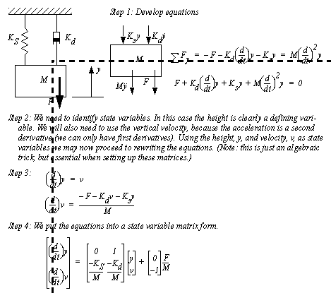

 

Figure 4.9 Example: Dynamic system

Figure 4.10 Example: Solving state equations with a TI-85 calculator shows the method for solving state equations on a TI-86 graphing calculator. (Note: this also works on other TI-8x calculators with minor modifications.) In the example a sinusoidal input force, F, is used to make the solution more interesting. The next step is to put the equation in the form expected by the calculator. When solving with the TI calculator the state variables must be replaced with the predefined names Q1, Q2, etc. The steps that follow describe the button sequences required to enter and analyze the equations. The result is a graph that shows the solution of the equation. Points can then be taken from the graph using the cursors. (Note: large solutions can sometimes take a few minutes to solve.)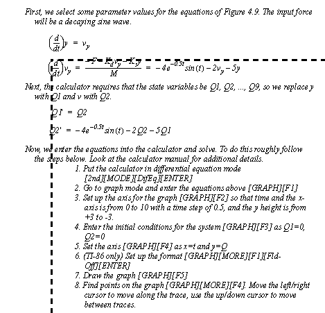

 

Figure 4.10 Example: Solving state equations with a TI-85 calculator

 

Figure 4.11 Example: Solving state equations with a TI-89 calculator

State equations can also be solved in Mathcad using built-in functions, as shown in Figure 4.12 Example: Solving state variable equations with Mathcad. The first step is to enter the state equations as a function, ’D(t, Q)’, where ’t’ is the time and ’Q’ is the state variable vector. (Note: the equations are in a vector, but it is not the matrix form.) The state variables in the vector ’Q’ replace the original state variables in the equations. The ’rkfixed’ function is then used to obtain a solution. The arguments for the function, in sequence are; the state vector, the start time, the end time, the number of steps, and the state equation function. In this case the 10 second time interval is divided into 100 parts each 0.1s in duration. This time is chosen because of the general response time for the system. If the time step is too large the solution may become unstable and go to infinity. A time step that is too small will increase the computation time marginally. When in doubt, run the calculator again using a smaller time step.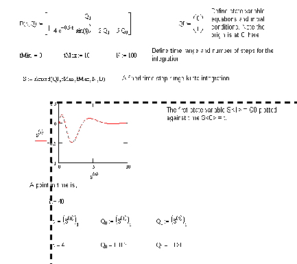

 

Figure 4.12 Example: Solving state variable equations with Mathcad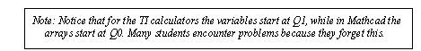

 

The simplest form of numerical integration is Euler’s first-order method. Given the current value of a function and the first derivative, we can estimate the function value a short time later, as shown in Figure 4.13 First-order numerical integration. (Note: Recall that the state equations allow us to calculate first-order derivatives.) The equation shown is known as Euler’s equation. Basically, using a known position and first derivative we can calculate an approximate value a short time, h, later. Notice that the function being integrated curves downward, creating an error between the actual and estimated values at time ’t+h’. If the time step, h, were smaller, the error would decrease.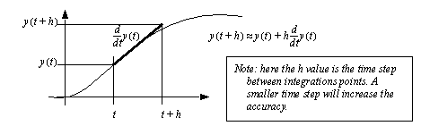

 

Figure 4.13 First-order numerical integration

The example in Figure 4.14 Example: First order numerical integration shows the solution of Newton’s equation using Euler’s method. In this example we are determining velocity by integrating the acceleration caused by a force. The acceleration is put directly into Euler’s equation. This is then used to calculate values iteratively in the table. Notice that the values start before zero so that initial conditions can be used. If the system was second-order we would need two previous values for the calculations.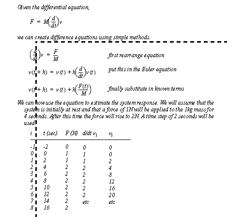

 

Figure 4.14 Example: First order numerical integration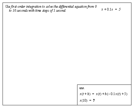

 

Figure 4.15 Drill problem: Numerically integrate the differential equation

An example of solving the previous example with a traditional programming language is shown in Figure 4.16 Example: Solving state variable equations with a C program. In this example the results will be written to a text file ’out.txt’. The solution iteratively integrates from 0 to 10 seconds with time steps of 0.1s. The force value is varied over the time period with ’if’ statements. The integration is done with a separate function.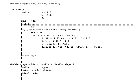

 

Figure 4.16 Example: Solving state variable equations with a C program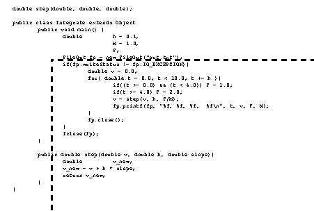

 

Figure 4.17 Example: Solving state variable equations with a Java program

The program in Figure 4.18 Example: First order integration with Scilab is for Scilab (a Matlab clone). The state variable function is defined first. This is followed by a definition of the parameters to be used for the numerical integration. Finally the function is solved explicitly (with the exact function).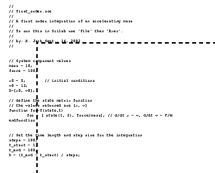

 

Figure 4.18 Example: First order integration with Scilab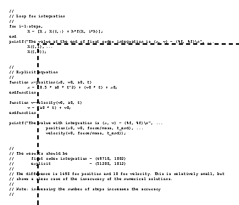

 

Figure 4.19 Example: First order integration with Scilab (continued)

First-order integration works well with smooth functions. But, when a highly curved function is encountered we can use a higher order integration equation. The Taylor series equation shown in Figure 4.20 The Taylor series for approximating a function. Notice that the first part of the equation is identical to Euler’s equation, but the higher order terms add accuracy.

 

Figure 4.20 The Taylor series

An example of the application of the Taylor series is shown in Figure 4.21 Example: Integration using the Taylor series method. Given the differential equation, we must first determine the derivatives and substitute these into Taylor’s equation. The resulting equation is then used to iteratively calculate values.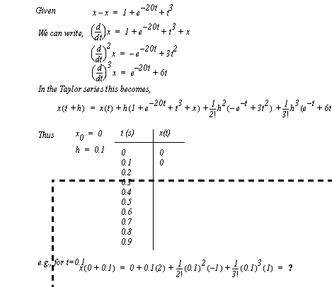

 

Figure 4.21 Example: Integration using the Taylor series method

Recall that the state variable equations are first-order equations. But, to obtain accuracy the Taylor method also requires higher order derivatives, thus making is unsuitable for use with state variable equations.

First-order integration provides reasonable solutions to differential equations. That accuracy can be improved by using higher order derivatives to compensate for function curvature. The Runge-Kutta technique uses first-order differential equations (such as state equations) to estimate the higher order derivatives, thus providing higher accuracy without requiring other than first-order differential equations.

The equations in Figure 4.22 Fourth order Runge-Kutta integration are for fourth order Runge-Kutta integration. The function ’f()’ is the state equation or state equation vector. For each time step the values ’F1’ to ’F4’ are calculated in sequence and then used in the final equation to find the next value. The ’F1’ to ’F4’ values are calculated at different time steps, and values from previous time steps are used to ’tweak’ the estimates of the later states. The final summation equation has a remote similarity to the first order integration equation. Notice that the two central values in time are more heavily weighted.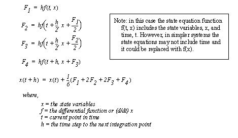

 

Figure 4.22 Fourth order Runge-Kutta integration

An example of a Runge-Kutta integration calculation is shown in Figure 4.23 Example: Runge-Kutta integration. The solution begins by putting the state equations in matrix form and defining initial conditions. After this, the four integrating factors are calculated. Finally, these are combined to get the final value after one time step. The number of calculations for a single time step should make obvious the necessity of computers and calculators.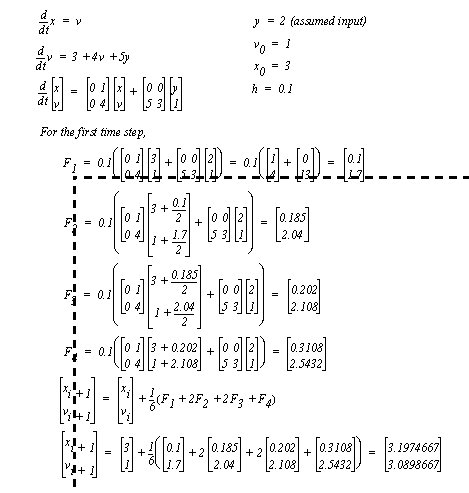

 

Figure 4.23 Example: Runge-Kutta integration

 

Figure 4.24 Drill problem: Integrate the acceleration function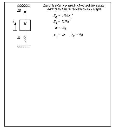

 

Figure 4.25 Drill problem: Integrate to find the system response

The program in Figure 4.26 Example: Runge-Kutta integration C program and Figure 4.28 Example: Runge-Kutta integration Scilab program is used to perform a Runge-Kutta integration of a mass-spring-damper system. The ’main’ program loops through the time steps and writes the value to a file. The ’step’ function performs one timestep integration for a second order Runge-Kutta integration. It uses the functions ’add’ and ’multiply’ to manipulate the state matrix. The ’derivative’ function updates the state matrix with the new derivative values.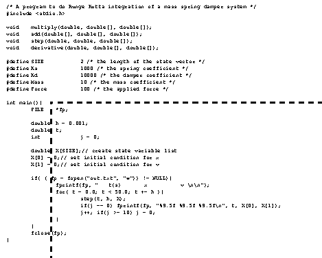

 

Figure 4.26 Example: Runge-Kutta integration C program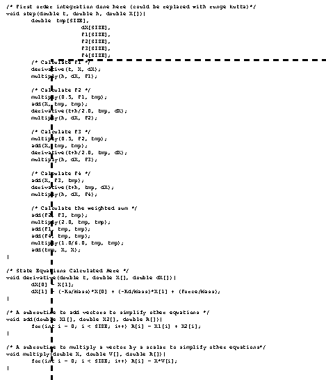

 

Figure 4.27 Example: Runge-Kutta integration C program (cont’d)

A Scilab program is given in Figure 4.28 Example: Runge-Kutta integration Scilab program to perform a Runge Kutta integration.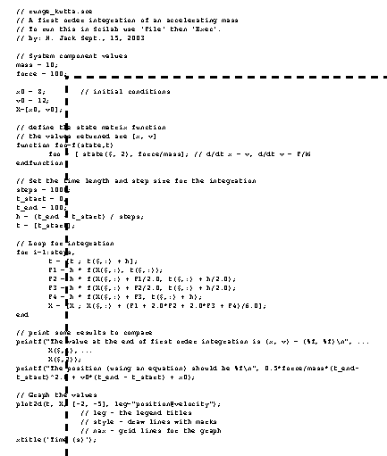

 

Figure 4.28 Example: Runge-Kutta integration Scilab program