RESPONSES

Solving differential equations tends to yield one of two basic equation forms. The e-to-the-negative-t forms are the first-order responses and slowly decay over time. They never naturally oscillate, and only oscillate if forced to do so. The second-order forms may include natural oscillation.

A first-order system is described with a first-order differential equation. The response function for these systems is natural decay or growth as shown in Figure 3.16 Typical first-order responses. The time constant for the system can be found directly from the differential equation. It is a measure of how quickly the system responds to a change. When an input to a system has changed, the system output will be approximately 63% of the way to its final value when the elapsed time equals the time constant. The initial and final values of the function can be determined algebraically to find the first-order response with little effort.

If we have experimental results for a system, we can calculate the time constant, initial and final values. The time constant can be found two ways, one by extending the slope of the first (linear) part of the curve until it intersects the final value line. That time at the intersection is the time constant. The other method is to look for the time when the output value has shifted 63.2% of the way from the initial to final values for the system. Assuming the change started at t=0, the time at this point corresponds to the time constant.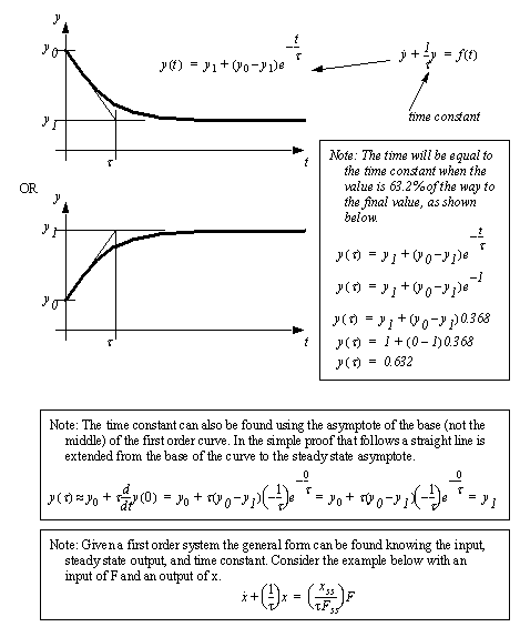

 

Figure 3.16 Typical first-order responses

The example in Figure 3.17 Example: Finding an equation using experimental data calculates the coefficients for a first-order differential equation given a graphical output response to an input. The differential equation is for a permanent magnet DC motor, and will be examined in a later chapter. If we consider the steady state when the speed is steady at 1400RPM, the first derivative will be zero. This simplifies the equation and allows us to calculate a value for the parameter K in the differential equation. The time constant can be found by drawing a line asymptotic to the start of the motor curve, and finding the point where it intercepts the steady-state value. This gives an approximate time constant of 0.8 s. This can then be used to calculate the remaining coefficient. Some additional numerical calculation leads to the final differential equation as shown.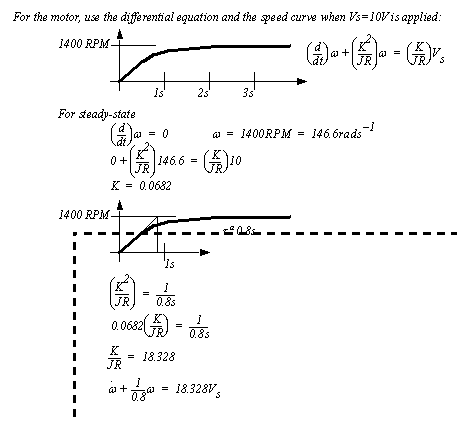

 

Figure 3.17 Example: Finding an equation using experimental data

 

Figure 3.18 Drill problem: Find the constants for the equation

A simple mechanical example is given in Figure 3.19 Example: First-order system analysis. The modeling starts with a FBD and a sum of forces. After this, the homogenous solution is found by setting the non-homogeneous part to zero and solving. Next, the particular solution is found, and the two solutions are combined. The initial conditions are used to find the remaining unknown coefficients.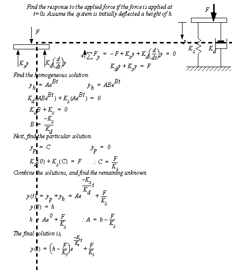

 

Figure 3.19 Example: First-order system analysis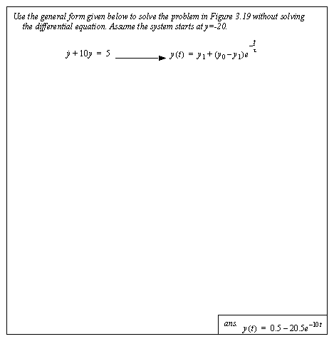

 

Figure 3.20 Drill problem: Developing the final equation using the first-order model form

A first-order system tends to be passive, meaning it doesn’t deliver energy or power. A first-order system will not oscillate unless the input forcing function is also oscillating. The output response lags the input and the delay is determined by the system’s time constant.

A second-order system response typically contains two first-order responses, or a first-order response and a sinusoidal component. A typical sinusoidal second-order response is shown in Figure 3.21 The general form for a second-order system. Notice that the coefficients of the differential equation include a damping factor and a natural frequency. These can be used to develop the final response, given the initial conditions and forcing function. Notice that the damped frequency of oscillation is the actual frequency of oscillation. The damped frequency will be lower than the natural frequency when the damping factor is between 0 and 1. If the damping factor is greater than one the damped frequency becomes negative, and the system will not oscillate because it is overdamped.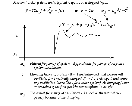

 

Figure 3.21 The general form for a second-order system

When only the damping factor is increased, the frequency of oscillation, and overall response time will slow, as seen in Figure 3.22 The effect of the damping factor. When the damping factor is 0 the system will oscillate indefinitely. Critical damping occurs when the damping factor is 1. At this point both roots of the differential equation are equal. The system will not oscillate if the damping factor is greater than or equal to 1.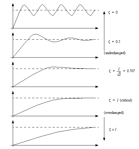

 

Figure 3.22 The effect of the damping factor

When observing second-order systems it is more common to use more direct measurements of the response. Some of these measures are shown in Figure 3.23 Characterizing a second-order response (not to scale). The rise time is the time it takes to go from 10% to 90% of the total displacement, and is comparable to a first order time constant. The settling time indicates how long it takes for the system to pass within a tolerance band around the final value. The permissible zone shown is 2%, but if it were larger the system would have a shorter settling time. The period of oscillation can be measured directly as the time between peaks of the oscillation, the inverse is the damped frequency. (Note: don’t forget to convert to radians.) The damped frequency can also be found using the time to the first peak, as half the period. The overshoot is the height of the first peak. Using the time to the first peak, and the overshoot the damping factor can be found.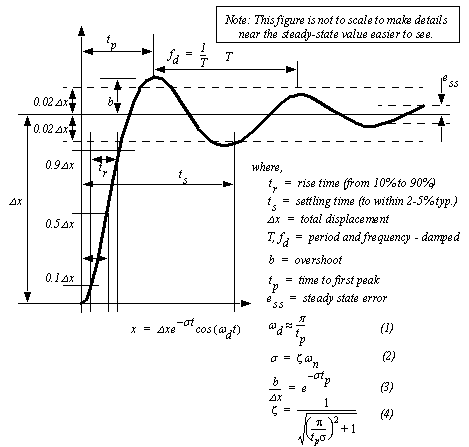

 

Figure 3.23 Characterizing a second-order response (not to scale)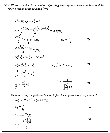

 

Figure 3.24 Second order relationships between damped and natural frequency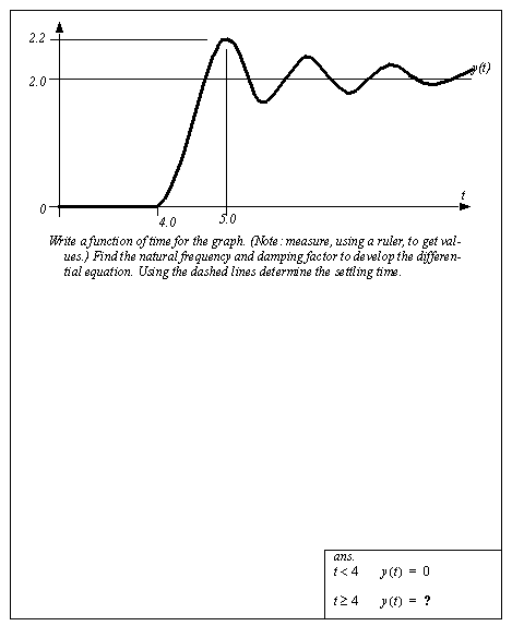

 

Figure 3.25 Drill problem: Find the equation given the response curve

First-order systems have e-to-the-t type responses. Second-order systems add another e-to-the-t response or a sinusoidal excitation. As we move to higher order linear systems we typically add more e-to-the-t terms, and/or more sinusoidal terms. A possible higher order system response is seen in Figure 3.26 An example of a higher order system response. The underlying function is a first-order response that drops at the beginning, but levels out. There are two sinusoidal functions superimposed, one with about one period showing, the other with a much higher frequency.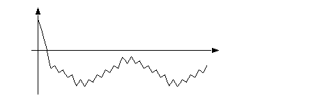

 

Figure 3.26 An example of a higher order system response

The basic techniques used for solving first and second-order differential equations can be applied to higher order differential equations, although the solutions will start to become complicated for systems with much higher orders. The example in Figure 3.27 Example: Solution of a higher order differential equation shows a fourth order differential equation. In this case the resulting homogeneous solution yields four roots. The result in this case are two real roots, and a complex pair. The two real roots result in e-to-the-t terms, while the complex pair results in a damped sinusoid. The particular solution is relatively simple to find in this example because the non-homogeneous term is a constant.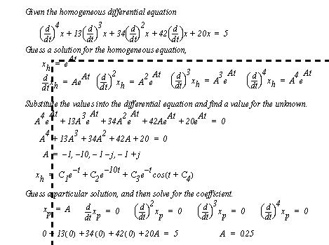

 

Figure 3.27 Example: Solution of a higher order differential equation

The example is continued in Figure 3.28 Example: Solution of a higher order differential equation and Figure 3.29 Example: Solution of a higher order differential equation (cont’d) where the initial conditions are used to find values for the coefficients in the homogeneous solution.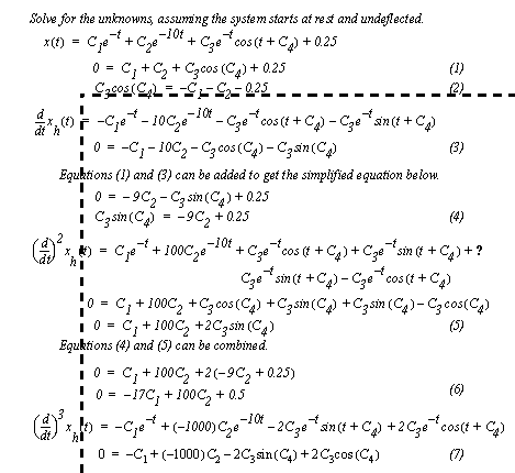

 

Figure 3.28 Example: Solution of a higher order differential equation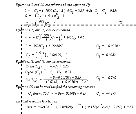

 

Figure 3.29 Example: Solution of a higher order differential equation (cont’d)

In some cases we will have systems with multiple differential equations, or non-linear terms. In these cases explicit analysis of the equations may not be feasible. In these cases we may use other techniques, such as numerical integration, which will be covered in later chapters.