There are two basic types of move functions;
MOV(value,destination) - moves a value to a memory location
MVM(value,mask,destination) - moves a value to a memory location, but with a mask to select specific bits.
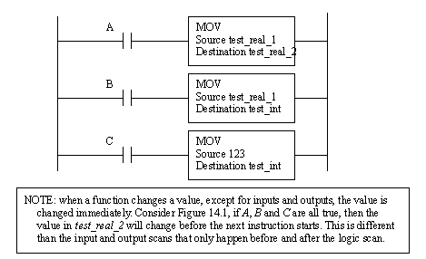
The simple MOV will take a value from one location in memory and place it in another memory location. Examples of the basic MOV are given in Figure 14.1 Examples of the MOV Function. When A is true the MOV function moves a floating point number from the source to the destination address. The data in the source address is left unchanged. When B is true the floating point number in the source will be converted to an integer and stored in the destination address in integer memory. The floating point number will be rounded up or down to the nearest integer. When C is true the integer value of 123 will be placed in the integer file test_int.

Figure 14.1 Examples of the MOV Function
A more complex example of move functions is given in Figure 14.1 Example of the MOV and MVM Statement with Binary Values. When A becomes true the first move statement will move the value of 130 into int_0. And, the second move statement will move the value of -9385 from int_1 to int_2. (Note: The number is shown as negative because we are using 2s compliment.) For the simple MOVs the binary values are not needed, but for the MVM statement the binary values are essential. The statement moves the binary bits from int_3 to int_5, but only those bits that are also on in the mask int_4, other bits in the destination will be left untouched. Notice that the first bit int_5.0 is true in the destination address before and after, but it is not true in the mask. The MVM function is very useful for applications where individual binary bits are to be manipulated, but they are less useful when dealing with actual number values.
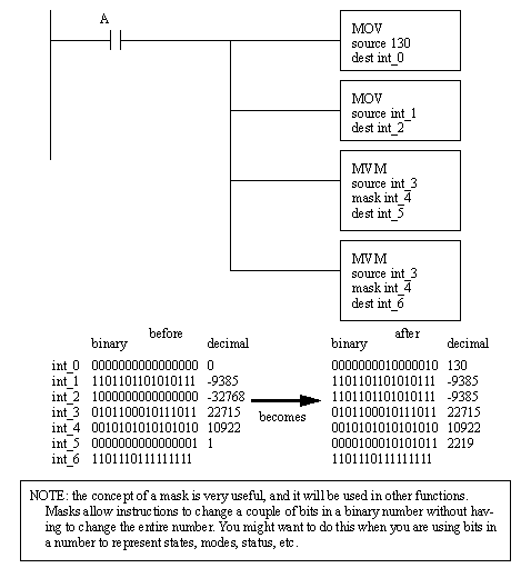
Figure 14.1 Example of the MOV and MVM Statement with Binary Values
Mathematical functions will retrieve one or more values, perform an operation and store the result in memory. Figure 14.1 Arithmetic Functions shows an ADD function that will retrieve values from int_1 and real_1, convert them both to the type of the destination address, add the floating point numbers, and store the result in real_2. The function has two sources labelled source A and source B. In the case of ADD functions the sequence can change, but this is not true for other operations such as subtraction and division. A list of other simple arithmetic function follows. Some of the functions, such as the negative function are unary, so there is only one source.
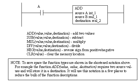
Figure 14.1 Arithmetic Functions
An application of the arithmetic function is shown in Figure 14.1 Arithmetic Function Example. Most of the operations provide the results we would expect. The second ADD function retrieves a value from int_3, adds 1 and overwrites the source - this is normally known as an increment operation. The first DIV statement divides the integer 25 by 10, the result is rounded to the nearest integer, in this case 3, and the result is stored in int_6. The NEG instruction takes the new value of -10, not the original value of 0, from int_4 inverts the sign and stores it in int_7.
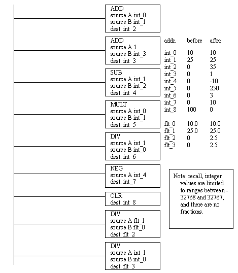
Figure 14.1 Arithmetic Function Example
A list of more advanced functions are given in Figure 14.1 Advanced Mathematical Functions. This list includes basic trigonometry functions, exponents, logarithms and a square root function. The last function CPT will accept an expression and perform a complex calculation.
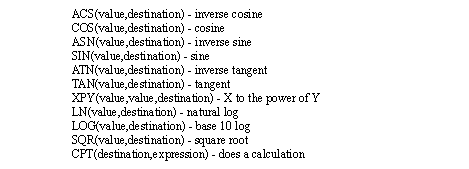
Figure 14.1 Advanced Mathematical Functions
Figure 14.1 An Equation in Ladder Logic shows an example where an equation has been converted to ladder logic. The first step in the conversion is to convert the variables in the equation to unused memory locations in the PLC. The equation can then be converted using the most nested calculations in the equation, such as the LN function. In this case the results of the LN function are stored in another memory location, to be recalled later. The other operations are implemented in a similar manner. (Note: This equation could have been implemented in other forms, using fewer memory locations.)
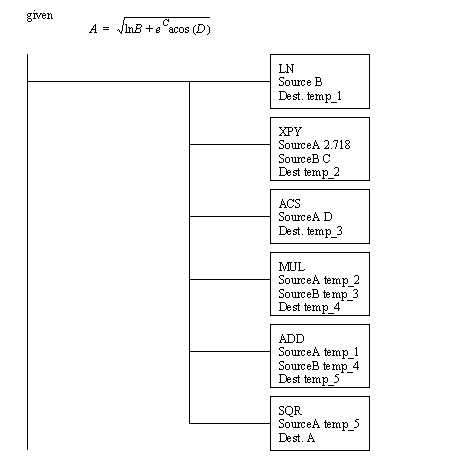
Figure 14.1 An Equation in Ladder Logic
The same equation in Figure 14.1 An Equation in Ladder Logic could have been implemented with a CPT function as shown in Figure 14.1 Calculations with a Compute Function. The equation uses the same memory locations chosen in Figure 14.1 An Equation in Ladder Logic. The expression is typed directly into the PLC programming software.

Figure 14.1 Calculations with a Compute Function
Math functions can result in status flags such as overflow, carry, etc. care must be taken to avoid problems such as overflows. These problems are less common when using floating point numbers. Integers are more prone to these problems because they are limited to the range.
Ladder logic conversion functions are listed in Figure 14.1 Conversion Functions. The example function will retrieve a BCD number from the D type (BCD) memory and convert it to a floating point number that will be stored in F8:2. The other function will convert from 2s compliment binary to BCD, and between radians and degrees.

Figure 14.1 Conversion Functions
Examples of the conversion functions are given in Figure 14.1 Conversion Example. The functions load in a source value, do the conversion, and store the results. The TOD conversion to BCD could result in an overflow error.
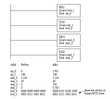
Figure 14.1 Conversion Example
Arrays allow us to store multiple data values. In a PLC this will be a sequential series of numbers in integer, floating point, or other memory. For example, assume we are measuring and storing the weight of a bag of chips in floating point memory starting at weight[0]. We could read a weight value every 10 minutes, and once every hour find the average of the six weights. This section will focus on techniques that manipulate groups of data organized in arrays, also called blocks in the manuals.
Functions are available that allow statistical calculations. These functions are listed in Figure 14.1 Statistic Functions. When A becomes true the average (AVE) conversion will start at memory location weight[0] and average a total of 4 values. The control word weight_control is used to keep track of the progress of the operation, and to determine when the operation is complete. This operation, and the others, are edge triggered. The operation may require multiple scans to be completed. When the operation is done the average will be stored in weight_avg and the weight_control.DN bit will be turned on.
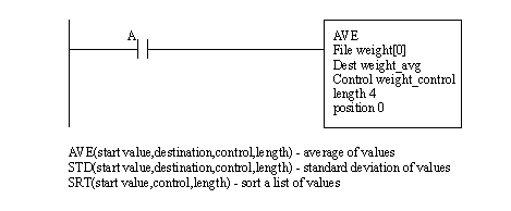
Figure 14.1 Statistic Functions
Examples of the statistical functions are given in Figure 14.1 Statistical Calculations for an array of data that starts at weight[0] and is 4 values long. When done the average will be stored in weight_avg, and the standard deviation will be stored in weight_std. The set of values will also be sorted in ascending order from weight[0] to weight[3]. Each of the function should have their own control memory to prevent overlap. It is not a good idea to activate the sort and the other calculations at the same time, as the sort may move values during the calculation, resulting in incorrect calculations.
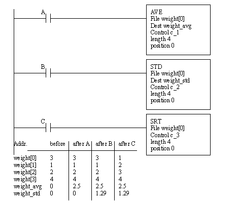
Figure 14.1 Statistical Calculations

A basic block function is shown in Figure 14.1 Block Operation Functions. This COP (copy) function will copy an array of 10 values starting at n[50] to n[40]. The FAL function will perform mathematical operations using an expression string, and the FSC function will allow two arrays to be compared using an expression. The FLL function will fill a block of memory with a single value.
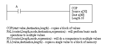
Figure 14.1 Block Operation Functions
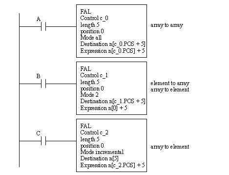
Figure 14.1 File Algebra Example shows an example of the FAL function with different addressing modes. The first FAL function will do the following calculations n[5]=n[0]+5, n[6]=n[1]+5, n[7]=n[2]+5, n[7]=n[3]+5, n[9]=n[4]+5. The second FAL statement will be n[5]=n[0]+5, n[6]=n[0]+5, n[7]=n[0]+5, n[7]=n[0]+5, n[9]=n[0]+5. With a mode of 2 the instruction will do two of the calculations when there is a positive edge from B (i.e., a transition from false to true). The result of the last FAL statement will be n[5]=n[0]+5, n[5]=n[1]+5, n[5]=n[2]+5, n[5]=n[3]+5, n[5]=n[4]+5. The last operation would seem to be useless, but notice that the mode is incremental. This mode will do one calculation for each positive transition of C. The all mode will perform all five calculations in a single scan whenever there is a positive edge on the input. It is also possible to put in a number that will indicate the number of calculations per scan. The calculation time can be long for large arrays and trying to do all of the calculations in one scan may lead to a watchdog time-out fault.
