5.1 DISCRETE SYSTEM MODELLING WITH EQUATIONS
������������
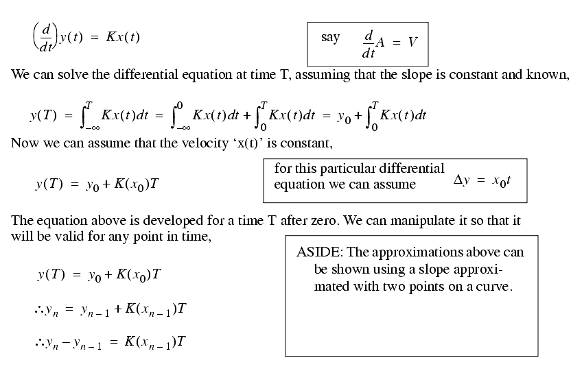
We can write a differential equation, and then manipulate it to put in terms of time steps of length `T'
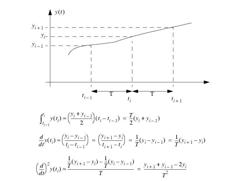
In review consider how we can approximate derivatives using two/three points on a line.
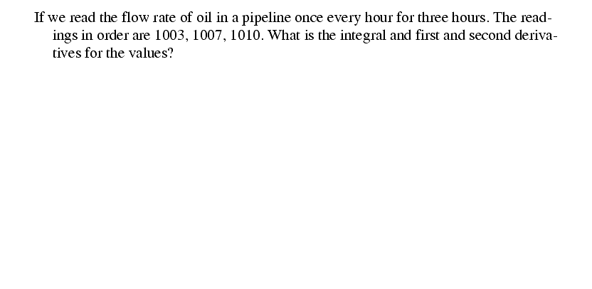
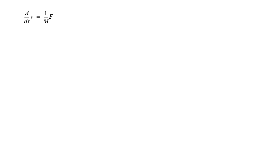
Consider the example,
5.1.1 Getting a Discrete Equation
������������
First, consider the example of a simple differential equation,
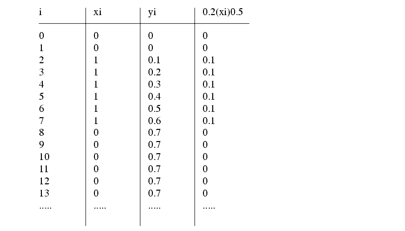
We can continue the example and use this equation to simulate the system. Here the `x' values are given, and the first `y' value is assumed to be 0. Assume T=0.5 and K=0.2.
Find the discrete equation for the differential equation below. Then find values over time.
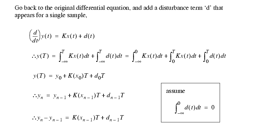
We can expand this model by also including a `disturbance'. This can be used to model random noise, or changes in system loading, found in all systems.
5.1.2 First Order System Example
������������
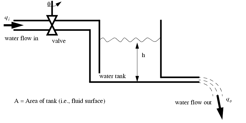
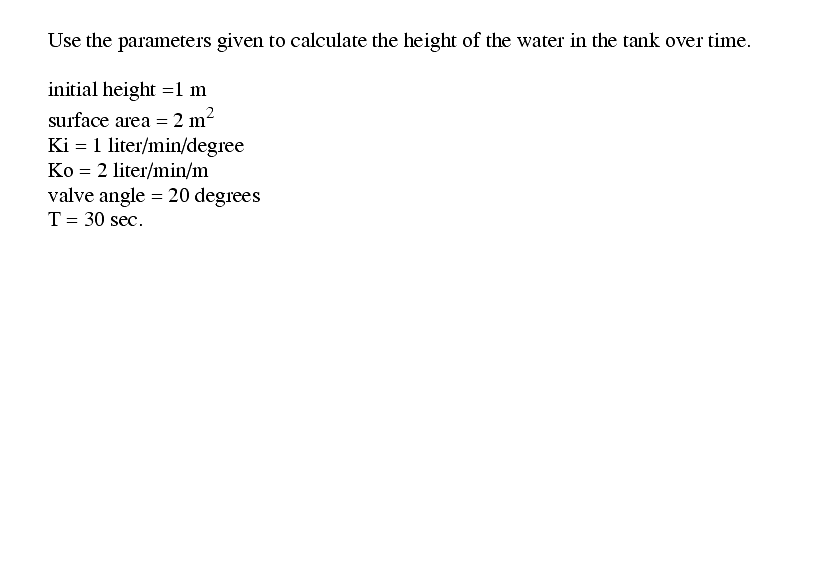
The water tank below has a small outlet, and left alone the fluid level in the tank will drop until empty. There is a valve controlled flow of fluids into the tank to raise the height of the fluid.
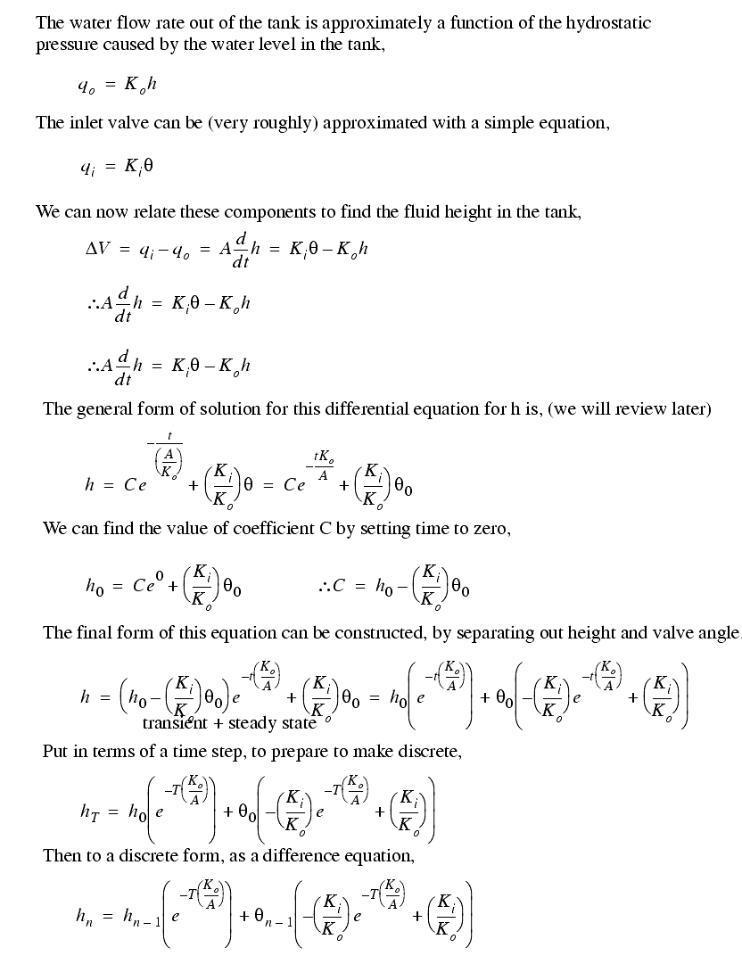
As long as the fluid levels in the tank are normal, the inlet and outlet flow rates are independent, We can model them both with simple differential equations,
This difference equation can then be used to predict fluid height. If we change the valve position, this will also be reflected in the calculated values.
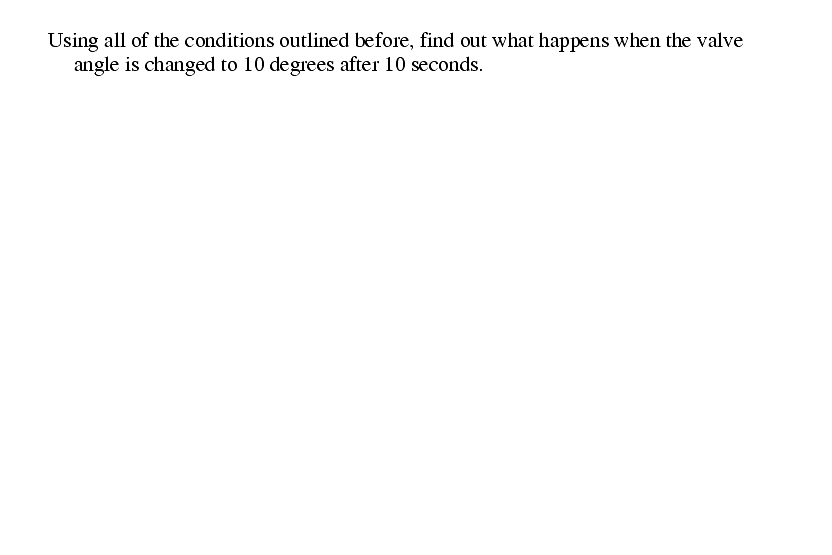
Now try varying the input valve angle,
5.1.3 Second Order System Example
������������
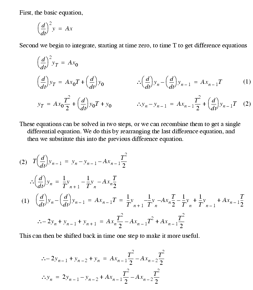
Consider the second order example below,
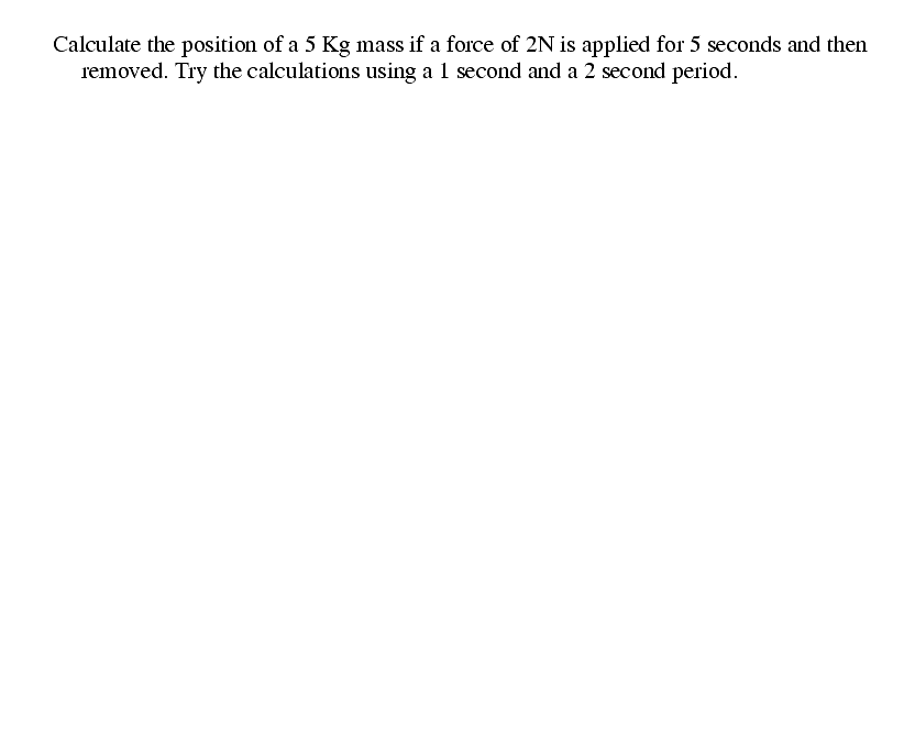
try the following problem.
5.1.4 Example of Dead (Delay) Time
������������
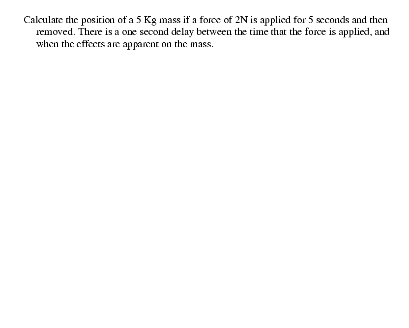
In a real system there is a distance between an actuator, and a sensor. This physical distance results to a lag between when we actuate something, and when the sensor sees a result.
Assume we have a simple process where after a change in x there is a delay of `m' time steps before the proportional change occurs in y. We can write the equation as,
Consider the example,

