14.1 STATE VARIABLE EQUATIONS

---

For analysis purposes it is useful to write the differential equations for a system in state variable form.

These equations will be in the form of first order differential equations. If they are not we will have to do some extra work to get them so that no derivative is higher than first order.

The term 'state' refers to variables that describe the current position of the system.

- these elements should be for energy storing elements (potential or kinetic).

- the variables must be independent.

- they should fully describe the system elements.

The state variable form is seen below,

Practice problem,

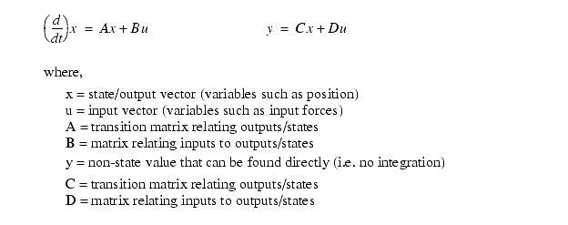
We want to select state variables that store energy. A capacitor voltage is a good choice, as is the position of an inertial mass or length of a spring. They both are the result of one or more integration steps.

The number of unknown values (state variables) must be the same as the number of equations to be able to solve the problem. This means that matrix A must be square.

Once the equations are in this form it is easy to integrate the values using a numerical technique such as Runge-Kutta integration.

The general approach to this technique is,

1. Generate the differential equations to model the process.

2. Select the state variables.

3. Rearrange the equations to state variable form.

4. Add additional equations as required.

5. Enter the problem into a computer and solve.

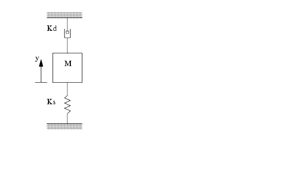
A simple example is given for a mass/spring combination.

The equations developed in step 3 can be used to solve the differential equations on most modern engineering calculators. For example on a TI-86 the basic steps are outlined in the example below.

To solve these problems in mathcad is a fairly similar method, and this can be seen in the figure below,

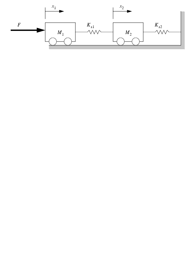
Develop the state variable form for the problem below,

Now solve the same problem with an added damper.

Develop the state variable form for the problem below,

Often we will get state equations that have more than one term with the same high order derivative. When this occurs we need to add a new dummy variable. (Note: This quite often happens for a sum of forces without a mass)

Consider the example below.

14.1.1 Numerical Integration

This form of integration is done numerically - this means by doing repeated calculations to solve the equation. Numerical techniques are not as elegant as solving differential equations, and will result in small errors. But these techniques make it possible to solve complex problems much faster.

This method uses forward/backward differences to estimate derivatives or integrals from measured data.

We can also estimate the change resulting from a derivative using Euler's equation for a first order difference equation. (This is known as the Euler method.)

Consider the following differential equation,

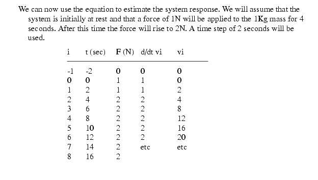
These methods can work well if the system is linear. But, if the system is not linear or the integration step is too long they will be very inaccurate.

14.1.2 Taylor Series

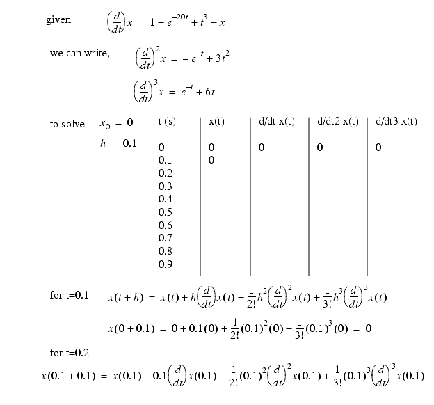
Recall the basic Taylor series,

We can integrate a given function as shown below,

14.1.3 Runge-Kutta Integration

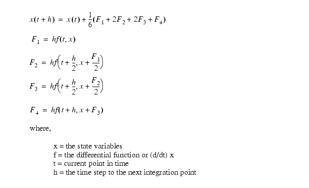
The equations below are for calculating a fourth order Runge-Kutta integration.

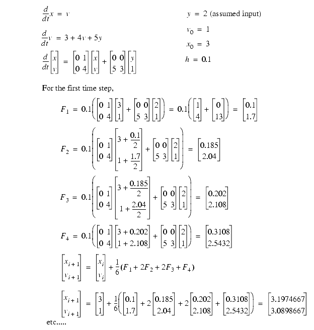
Integrate the functions below and use a time step of 0.1.

Mathcad, Working Model and all other computer based mathematics packages use this or a similar method for solving differential equations.

Try the practice problem below,

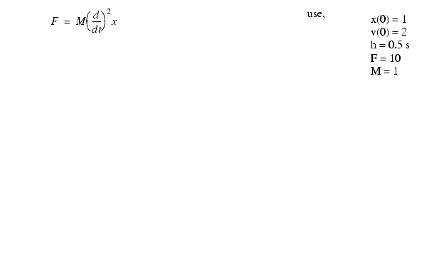
Try to simulate the system below using runge-kutta.