• Consider the basic transform tables. A superficial examination will show that the denominator (bottom terms) are the main factor in determining the final form of the solution. To explore this further, consider that the roots of the denominator directly impact the partial fraction expansion and the following inverse Laplace transfer.
• When designing a controller with variable parameters (typically variable gain), we need to determine if any of the adjustable gains will lead to an unstable system.
• Root locus plots allow us to determine instabilities (poles on the right hand side of the plane), overdamped systems (negative real roots) and oscillations (complex roots).
• Note: this procedure can take some time to do, but the results are very important when designing a control system.

• Consider the previous example, the transfer function for the whole system was found, but then only the denominator was used to determine stability. So in general we do not need to find the transfer function for the whole system.


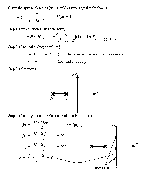
• The basic procedure for creating root locus plots is,
1. write the characteristic equation. This includes writing the poles and zeros of the equation.

2. count the number of poles and zeros. The difference (n-m) will indicate how many root loci lines end at infinity (used later).
3. plot the root loci that lie on the real axis. Points will be on a root locus line if they have an odd number of poles and zeros to the right. Draw these lines in.
4. determine the asymptotes for the loci that go to infinity using the formula below. Next, determine where the asymptotes intersect the real axis using the second formula. Finally, draw the asymptotes on the graph.

5. the breakaway and breakin points are found next. Breakaway points exist between two poles on the real axis. Breakin points exist between zeros. to calculate these the following polynomial must be solved. The resulting roots are the breakin/breakout points.

6. Find the points where the loci lines intersect the imaginary axis. To do this substitute the fourier frequency for the laplace variable, and solve for the frequencies. Plot the asymptotic curves to pass through the imaginary axis at this point.

• Consider the example in the previous section,


• Plot the root locus diagram for the function below,
