
|
|
|
3.1 DATA DISTRIBUTIONS

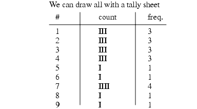
3.1.1 HISTOGRAMS
Histograms can be used to show these distributions graphically.


Cumulative distributions can be used to estimate the probability of an event. For example, if in the graph above we want to know how many pizzas are delivered within 25 minutes, we could read 10 (approx.) every week off the graph.
there are typically 10 to 20 divisions in a histogram
percentages can be used on the right axis, in place of counts.
3.1.2 Continuous Distributions
Histograms are useful for grouped data, but in the cases where the data is continuous, we use distributions of probability.
In specific, some of the distribution properties are,
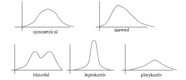
In addition the centre of the distribution can vary (i.e. the average or mean)
3.1.3 Describing Distribution Centres With Numbers
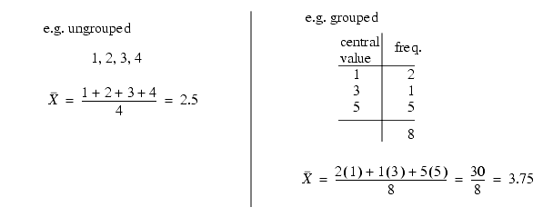
The best known method is the average. This gives the centre of a distribution


Another good measure is the median

If the numbers are grouped the median becomes

Mode can be useful for identifying repeated patterns

3.1.4 Dispersion As A Measure of Distribution
The range of values covered by a distribution are important

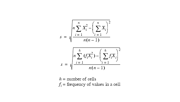
Standard deviation is a classical measure of grouping (for normal distributions??????????)


When we use a standard deviation, we can estimate the distribution of the samples.

By adding standard deviations to increase the range size, the percentage of samples included are,

Other formulas for standard deviation are,
3.1.5 The Shape of the Distribution

this lack of symmetry tends to indicate a bias in the data (and hence in the real world)
a skew factor can be calculated

3.1.6 Kurtosis

This is best used for comparison to other values. i.e. you can watch the trends in the values of a4.
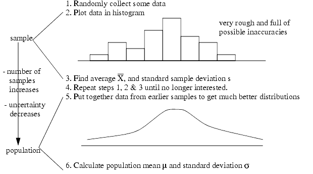
3.1.7 Generalizing From a Few to Many
3.1.8 The Normal Curve
this is a good curve that tends to represent distributions of things in nature (also called Gaussian)
This distribution can be fitted for populations (m, s), or for samples (X, s)
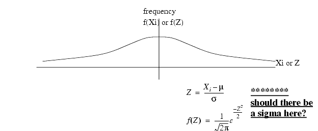
The area under the curve is 1, and therefore will enclose 100% of the population.
the parameters vary the shape of the distribution

The area under the curve indicates the cumulative probability of some event

When applied to quality ±3s are used to define a typical "process variability" for the product. This is also known as the upper and lower natural limits (UNL & LNL)
READ or REVIEW: chapter 3, pg 43-93
PROBLEMS: pg 93- #4, 8, 17, 18, 21, 23, 25, 28, 30, 40
******************* LOOK INTO USE OF SYMBOLS, and UNL, LNL, UCL, LCL, etc.
3.1.9 Probability plots


READING: chapter 4, pg. 103-165
Search for More: |

Custom Search
|

|