2. Statistics
• Why?
Because we can’t sample every part.
Because no matter what we do, no two parts will be the same.
Because we define a product to meet specifications and we can measure how well it conforms.
Because differences between parts are hard (assignable causes) or impossible (chance causes) to predict.
Because we can sample a few and draw conclusions about the whole group.
• What is the objective?
We want to sample as little data as possible to draw the most accurate conclusions about the distribution of the values.
• Two type of statistics
Inductive: Try to get overall variance within group. i.e. assume all of group should conform ***WE USE THIS TYPE
Deductive: Attempt to classify differences that exist within a group (i.e. election polls).
2.1 Data Distributions
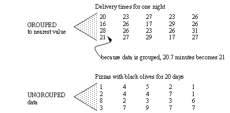
• Showing Differences
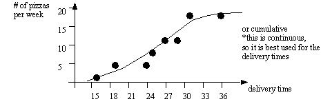
consider Domino’s pizza that delivered < 30minutes by tolerance
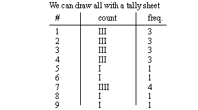
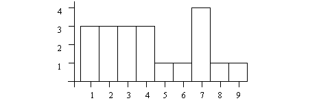
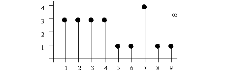
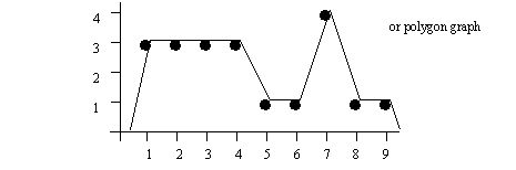
2.1.1 Histograms
• Histograms can be used to show these distributions graphically.
• Cumulative distributions can be used to estimate the probability of an event. For example, if in the graph above we want to know how many pizzas are delivered within 25 minutes, we could read 10 (approx.) every week off the graph.
• there are typically 10 to 20 divisions in a histogram
• percentages can be used on the right axis, in place of counts.
2.1.2 Continuous Distributions
• Histograms are useful for grouped data, but in the cases where the data is continuous, we use distributions of probability.
• In general
the area under the graph = 1.00000.......
the graphs often stretch (asymptotically) to infinity
• In specific, some of the distribution properties are,
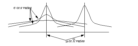
• In addition the center of the distribution can vary (i.e. the average or mean)
• More on distribution later
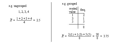
2.1.3 Describing Distribution Centers With Numbers
• The best known method is the average. This gives the center of a distribution
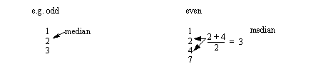
• Another good measure is the median
If odd number of samples it is the middle number
If an even number of samples, it is the average of the left and right bounding numbers
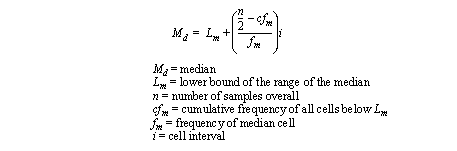
• If the numbers are grouped the median becomes
• Mode can be useful for identifying repeated patterns
a mode is a repeated value that occurs the most. Multiple modes are possible.
2.1.4 Dispersion As A Measure of Distribution
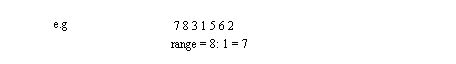
• The range of values covered by a distribution are important
Range is the difference between the highest and lowest numbers.
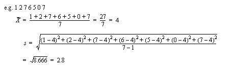
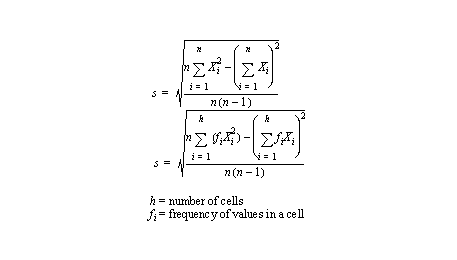
• Standard deviation is a classical measure of grouping (for normal distributions??????????)
the equation is,
• When we use a standard deviation, we can estimate the distribution of the samples.
• By adding standard deviations to increase the range size, the percentage of samples included are,
• Other formulas for standard deviation are,
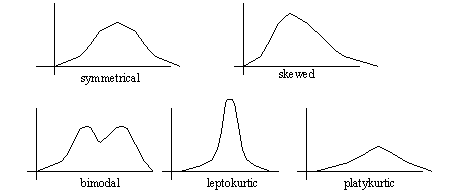
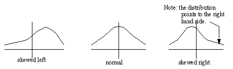
2.1.5 The Shape of the Distribution
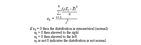
• Skewed functions
• this lack of symmetry tends to indicate a bias in the data (and hence in the real world)
• a skew factor can be calculated
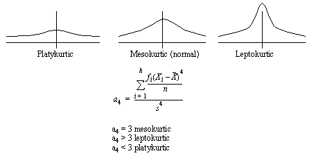
2.1.6 Kurtosis
• This is a peaking in the data
• This is best used for comparison to other values. i.e. you can watch the trends in the values of a4.
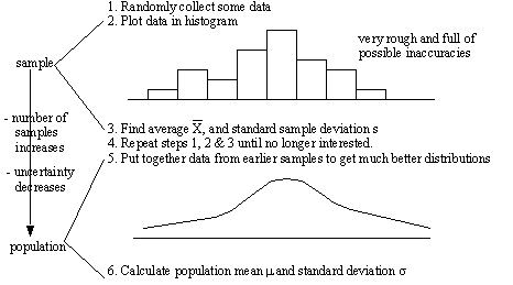
2.1.7 Generalizing From a Few to Many
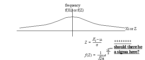
2.1.8 The Normal Curve
• this is a good curve that tends to represent distributions of things in nature (also called Gaussian)
• This distribution can be fitted for populations (μ, σ), or for samples (X, s)
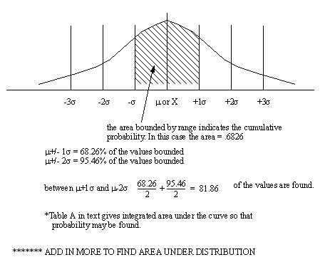
• The area under the curve is 1, and therefore will enclose 100% of the population.
• the parameters vary the shape of the distribution
• The area under the curve indicates the cumulative probability of some event
• When applied to quality ±3σ are used to define a typical “process variability” for the product. This is also known as the upper and lower natural limits (UNL & LNL)
******************* LOOK INTO USE OF SYMBOLS, and UNL, LNL, UCL, LCL, etc.
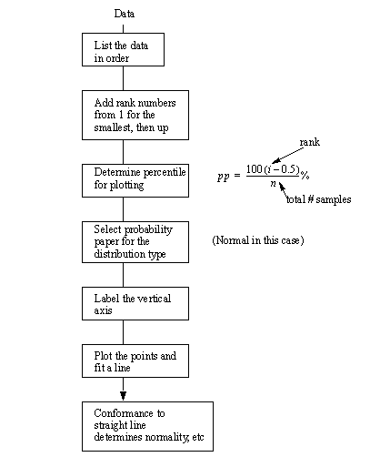
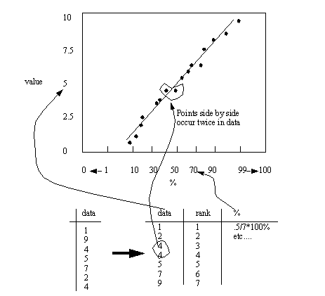
2.1.9 Probability plots
• Procedure
2.2 Probability
• A way to figure out how chances interact
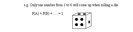
• Mutually Exclusive: Probable events can only happen as one or the other.
• Not Mutually Exclusive: Probable events can occur simultaneously
• Independent Probabilities: Events will happen separately
• Dependant Probabilities: The outcome of one event effects the outcome of another event
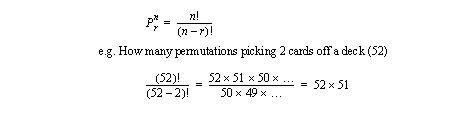
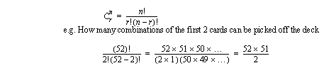
• Permutations: for exact definitions of not only possibilities, but also order.
• Combinations: similar to before except order does not mater.
• empirical probability: experimentally determine the probability with,
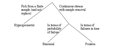
2.2.1 Discrete Distributions
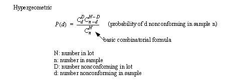
2.2.2 Hypergeometric Distribution
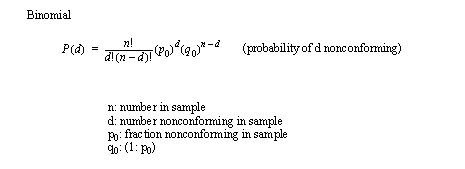
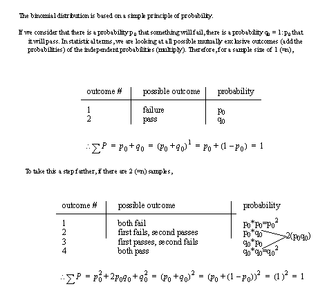
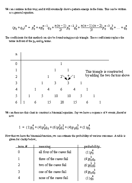
2.2.3 Binomial Distribution
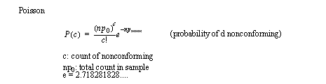
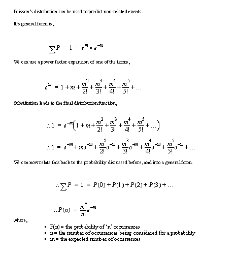
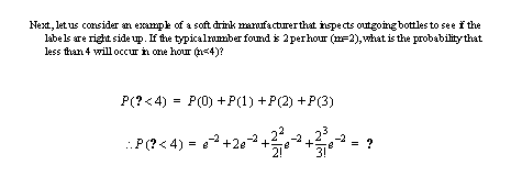
2.2.4 Poisson Distribution