H. Jack (member), D. M. A. Lee (member), R O. Buchal (member), W. H. ElMaraghy, The University of Western Ontario, Department of Mechanical Engineering, London, Ontario, Canada, N6A 5B9

I. Introduction

Over the past decade, the artificial intelligence community has undergone a resurgence of interest in the research and development of artificial neural networks. An artificial neural network is an attempt to simulate the manner in which the brain interprets information as determined by the current knowledge of biology, physiology, and psychology [14]. Artificial neural networks behave in much the same manner as biological neural networks, giving many of the same benefits. Artificial neural nets are fault tolerant, exhibit the ability to learn and adapt to new situations, and have the ability to generalize based on a limited set of data. This arises because of the structure which allows neural nets to process information simultaneously, as opposed to the serial nature of traditional digital computers. This parallel nature, inherent in neural networks, achieves the increase in speed by distributing the calculations among many neurons. The network structure provides a level of fault tolerance, which allows the network to withstand component failures without having the entire network fail.

This paper focuses on a popular feedforward model of neural networks. In this model a set of inputs are applied to the network, and multiplied by a set of connection weights. All of the weighted inputs to the neuron are then summed and an activation function is applied to the summed value. This activation level becomes the neuron’s output and can be either an input for other neurons, or an output for the network. Learning in this network is done by adjusting the connection weights based upon training vectors (input and corresponding desired output). When a training vector is presented to a neural net, the connection weights are adjusted to minimize the difference between the desired and actual output. After a network is trained with a set of training vectors, the network should produce a good output match for the inputs.

Artificial neural networks are mainly used in two areas --- pattern recognition, and pattern matching. Pattern recognition is performed by classifying an unknown pattern through comparisons with previously learned patterns. This ability is termed associative recall. An example of this is the use of neural networks to recognize handwritten digits [4]. In pattern recognition, when a particular pattern is noisy or distorted, the network can generalize and choose the closest match [3][4][10][13]. Pattern matching uses continuous input patterns to evoke continuous output patterns (i.e. one-to-one mappings). An example is the use of a neural network as a basic controller for a plant. The controller would accept the plant conditions as the inputs, and a set of control outputs would drive the current manufacturing process. This approach is discussed in more detail in [11]. This paper uses the pattern matching strategy for the inverse kinematics of a typical three link manipulator.

This paper focuses on the kinematic control of a three link manipulator working in three dimensional space, within a quarter of the robot workspace. When manipulators interact with the environment, the position of the end effector must be described. Human users are more suited to working in cartesian coordinates than the joint coordinates of robots; hence, there is a need for conversion between the two coordinate systems. The conversion from world coordinates to robot joint angles is called inverse kinematics. In the past, the problem of solving the inverse kinematics has been done through the application of various methods. These methods take one of two basic forms (i) Closed form equations or, (ii) Iterative. A closed form solution is found by decoupling the joints responsible for position and those responsible for orientation. These solution types are more desirable since explicit equations are available. Iterative techniques, such as, Newton-Raphson, Newton-Gauss and Linearization are available when no closed form solutions can be obtained. Many of these solutions require that the kinematics be performed off-line because of the computational demands of the algorithms. A brief survey of these various algorithms is given in [2] and [15]. Both of the forms are generally rigid and do not account for uncontrollable variables such as manufacture tolerances, calibration error, and wear. A neural network approach could adapt to changes in the robot due to wear from extended use over time. Such algebraic and algorithmic procedures cannot incorporate these situations.

Previous research in the application of neural networks to kinematic control was performed for a to a two-link planar manipulator (working in a plane), and a five degree of freedom robot working in three dimensional space. The manipulators were controlled with a high accuracy; however, the training region for the two link robot was a small square in the center of the workspace, and the five link robot was limited to a small wedge volume within the robot workspace [5][6][7]. This paper explains research extended to investigate the performance throughout the entire work space of the robot. Investigations of a more complete representation of inverse kinematics throughout the entire workspace is provided.

The paper begins with a general introduction to the artificial neuron, a brief description of feedforward neural networks, and a description of the backpropagation learning algorithm. The inverse kinematics problem is described, and the application of a two-layer neural network is discussed. The use of compensation networks is explored and the results of the experimental work are presented. The implications of the neural network approach to the kinematic control problem are presented at the conclusion of this paper.

II. The Basic Artificial Neuron

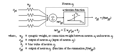
The basic building block of an artificial neural network is the neuron. In a popular model which will be used in this paper, the connection weights between neurons are adjusted. The neuron receives inputs opi from neuron ui while the network is exposed to input pattern p. Each input is multiplied by a connection weight wij, where wij is the connection between neurons ui and uj. The connection weights correspond to the strength of the influence of each of the preceding neurons. After the inputs have been multiplied by the connection weights for input pattern p, their values are summed, netpj. Included in the summation is a bias value θj to offset the basic level of the input to the activation function, f(netpj), which gives the output opj . Figure 1 shows the structure of the basic neuron.

Figure 1 Basic structure of an artificial neuron.

In order to establish a bias value θj, the bias term can appear as an input from a separate neuron with a fixed value (a value of +1 is common). Each neuron requiring a bias value will be connected to the same bias neuron. The bias values are then self-adjusted as the other neurons learn, without the need for extra considerations.

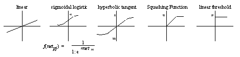
In calculating the output of the neuron, the activation function may be in the form of a threshold function, in which the output of the neuron is +1 if a threshold level is reached and 0 otherwise. Squashing functions limit the linear output between a maximum and minimum value. These linear functions, however, do not take advantage of multi-layer networks [14]. Hyperbolic tangents and the sigmoidal functions are similar to real neural responses; however, the hyperbolic tangent is unbounded and hard to implement in hardware. In this paper, the Sigmoidal function is used because of its ability to produce continuous non-linear functions, which can be implemented in hardware in future research areas. Figure 2 shows some commonly used activation functions.

Figure 2 Common activation functions.

For more in depth information on neural networks, please refer to introductions to the subject in [3], [8], [14] and [16].

III. Neural Network Architectures in Feedforward Systems

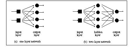
A single neuron can only simulate 14 of the 16 basic boolean logic functions. It cannot emulate the X-OR, or the X-NOR gates [9]. These limitations require that more than a single neuron be used, and thus, the architecture becomes an important consideration. In Feedforward systems, networks propagate the inputs forward through the neural net. Each neuron has inputs that only come from neurons in preceding layers. A one-layer neural net consists of a layer of input neurons and a layer of output neurons. A multi-layer network consists of an input layer of neurons, one or more hidden layers, and an output layer.

The circular nodes in figure 3 represent basic neurons, as described in the previous section. The input neurons are shown as squares because they only act as terminal points (i.e. opi = input). The input layer does not process information; thus, it is not considered to be a part of the structure and is numbered layer 0. A simple one-layer network can effectively map many sets of inputs to outputs. In pattern recognition problems, this depends upon the linear separability of the problem domain. In pattern matching problems, this depends upon continuity, and topography of the function. If such a set of connection weights cannot be found using one-layered networks, then multi-layered networks must be considered.

Figure 3 Simple feedforward artificial neural networks.

IV. Backpropagation of Errors

Learning methods may be either supervised, or unsupervised. Supervised learning is required for pattern matching, and backpropagation is the most popular of the supervised learning techniques. In the backpropagation Training Paradigm, the connection weights are adjusted to reduce the output error. In the initial state, the network has a random set of connection weights. When a system starts with all connection weights equal, the network begins at a sort of local optimum, and will not converge to the global solution. In order for the network to learn, a set of inputs are presented to the system and a set of outputs are calculated. A difference between the actual outputs and desired outputs is calculated and the connection weights are modified to reduce this difference [14].

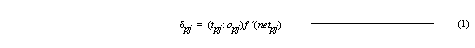
After inputs have been applied and the network output solution has been calculated, the estimated error contribution, δ, by each neuron must be calculated. The calculations begin at the output layer of the network. The delta value for any output neuron is computed as,

where, tpj is the desired output of output neuron uj, and opj is the actual output, and f ´(netpj) is the first derivative of the activation function with respect to the total input (netpj) for the given input pattern p evaluated at neuron uj.

For the output layer, the change in connection weights can easily be calculated since the δ of the output neurons is easily determined. With the introduction of hidden layers, the desired outputs of these hidden neurons becomes more difficult to estimate. In order to estimate the delta of a hidden neuron, the error signal from the output layer must be propagated backwards to all preceding layers. The delta, δpj , for the hidden neurons is calculated as,

where, f ´(netpj) is the first derivative of the activation function with respect to netpj at hidden neuron uj, δpk is the delta value for the subsequent neuron uk, and wjk is the connection weight for the link between hidden neuron uj and subsequent neuron uk. This process of calculating the δs is performed for all layers until the input layer is reached

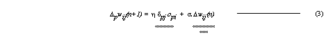
After all the error terms have been calculated for all the neurons, the weights may be adjusted. The estimated weight change Δpwij(n+1) is calculated for each input connection to neuron uj from neuron ui by,

where η is the learning rate, α is the smoothing term, δpj is the delta of neuron uj, opi is the output of preceding neuron ui, and Δwij(n) is the weight change in the previous training interval. The estimated errors are used to estimate the weight changes with the least mean squares method.

The backpropagation method is essentially a gradient descent approach which minimizes the errors. In order to adjust the connection weights, the gradient descent approach requires that steps be taken in weight space. If the steps are too large, then the weights will overshoot their optimum values. If the steps are too small, it may take longer to converge and may become caught in local minima. The step size is then a function of the learning rate. The learning rate, which varies between 0 and 1, should be large enough to come up with a solution in a reasonable amount of time without having the solution oscillate within weight space. By introducing the momentum term, which varies between 0 and 1, the learning rate can be increased while preventing oscillation. The momentum term is introduced by adding to the weight change some percentage of the last weight change. Common values for η range from 0.1 to 0.9, and common values of α range from 0.2 to 0.8

The training set is comprised of points which have inputs and desired outputs, which may or may not be in a random order. In this paper, the training points were chosen at random from an ordered table. This allows a weight correction after each point is trained. This method helps avoid local optimum points in weight space, by creating a random walk type of weight optimization, and gives a much faster global convergence. This process is then repeatedly performed for all training examples until a satisfactory output error is achieved. For an in-depth derivation of the back propagation method, the reader is suggested to consult Rumelhart and McClelland [14].

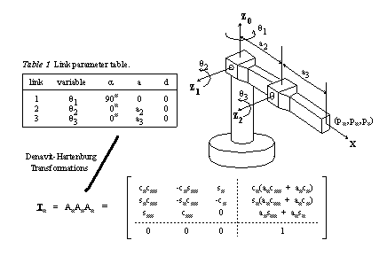
V. A Typical Three Link Manipulator

In order for a robotic manipulator to perform tasks within space, a user must specify a location in three dimensional space. The robotic controller must then determine the correct joint coordinates to locate the manipulator. This area of robotics, Inverse Kinematics, has been well researched and many good solutions exist. In all cases the resultant solutions are highly specific to a particular robot configuration, with exact dimensions. Such explicit solutions do not tolerate changes over time. These changes may be caused by poor tolerances in manufacture, wear over extended periods of operation, damage to the robot, and poor calibration. Computations are often complex, can be quite slow, and require a computer capable of performing complex mathematical functions.

An example of a robot which may be used with an artificial neural network control system is the three link manipulator as shown in figure 4. The forward and inverse kinematic equations, used by the authors in testing, are given in the equations (4) and (5).

Figure 4 A typical three link manipulator.

The ± sign in θ2 indicates the general configuration of the robot arm. The positive sign (+ve) corresponds to an elbow down solution, and the negative sign (-ve) corresponds to an elbow up solution.

It should be noted that the inverse kinematics is not determinate. The sources of indeterminacy for this manipulator occur:

for Elbow up and Elbow Down Configurations, and

when the end of the arm is directly over the origin, θ1 is undefined.

Other examples of indeterminacy occur in PUMA style robots where left and right arm configurations would give indeterminacy. These sources of indeterminacy may all be overcome by constraining the inverse kinematics to a particular case.

VI. Training a Neural Network for Inverse Kinematics

Neural Network solutions have the benefit of having faster processing times since information is processed in parallel. The solutions may be adaptive and still be implemented in hardware by using specialized electronics. Neural systems can generalize to approximate solutions from small training sets. Neural systems are fault tolerant and robust. The network will not fail if a few neurons are damaged, and the solutions may still retain accuracy. When implementing a neural network approach, complex computers are not essential and robot controllers need not be specific to any one manipulator.

The nature of neural networks require that a set of training points be chosen which represent the nature of the inputs (x, y, z) and the corresponding outputs (θ1, θ2 and θ3). If the training points chosen tend to be clustered, then the network will be very accurate when dealing with points near the cluster. In this case, the robot should be familiar with points throughout the entire workspace; thus, points should be evenly distributed. The order in which points are presented to the network also affect the speed and quality of convergence. If the points are not presented in a random order, each training update will tend to train the network for the current section of space which the points are from.

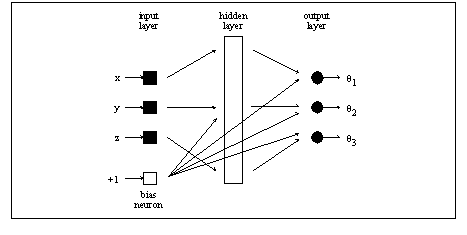
The neural network architecture chosen for this problem is a simple network with one hidden layer. The network has three input neurons for the desired position, and three output neurons for the estimated joint angles. A bias neuron (with a value of +1) is attached to all of the neurons in the hidden layer, and to all of the output neurons. The number of neurons in the hidden layer varied from 10, 20, and 40. This network architecture is pictured in figure 5.

Figure 5 Neural architecture for solving the inverse kinematic problem. For simplicity, the network is shown with a small amount of arrows; however, the network is actually fully connected.

It is expected that because the network is estimating the joint angles, there will be some errors involved. The value of the errors will vary over the work space and can be corrected by implementing secondary compensation neural networks. To calculate the joint coordinates, the main neural network was trained. After training the main network, the discrepancy between the network results and the actual values were found and those errors were used to train a second network for correction. The second network is referred to as a compensation network, and had an identical architecture to the main network. If both the main and compensation networks calculate an output estimate and a correction estimate, there will be yet another smaller error. Another network can then be set up to estimate this smaller error, and the accuracy of the solution may be improved further. Accuracy does improve as more correction networks are used. This paper tested a total of five correction networks. Please note that each of the networks was trained separately, one after another. Also note that the outputs from the networks are multiplied to scale the outputs up. The scaling factors on the outputs of each of the nets was made successively smaller.

Instead of gathering experimental information from a robot, the Inverse Kinematic equations were used. The use of simulated data provided a reliable training and comparison for the neural network. In order for the neural network to generalize to a one-to-one mapping, the training set consisted of a single solution set. To overcome the indeterminacy in the solution, a few assumptions were made:

elbow up was assumed (for the elbow down solution, a separate network would need to be considered)

the region above the origin was not used for training, to avoid the singularities at this location

the robot was trained over a one quarter sphere volume of the entire workspace (90o > θ1 > 0o). Training within a quarter of the workspace is valid because of the symmetry of the robot workspace

The decision to train over a quarter of the work sphere was based upon the premise that by limiting the scatter of the training points, the most accurate inverse kinematics mapping would be acquired. If the training set had covered the entire work space, then the solution may have been poorer with longer convergence times, because the network would have been forced to generalize over a volume which is four times larger.

VII. Performance of a Neural Network for Inverse Kinematics

All configurations tested were feedforward using the sigmoidal activation function. One hidden layer was used with the number of hidden neurons in the layer at 10, 20, and 40. The network converged slowly to a less than optimal solution when no bias was applied to the neurons in the hidden layer. Networks were tested with and without the bias neurons on the output neurons, with no noticeable difference, so, a bias was applied to every hidden neuron, and to every output neuron. The compensation networks had the exact same configuration as the original network.

For all of the data presented, the learning rate was set to 0.9, and the smoothing rate was set to 0.8. The number of iterations was set to be very high (the order of thousands) so that all of the network results should be at their optimum configuration. The training periods were performed on a SUN Sparcstation 1, taking times from 1 to 10 hours. All of the programs have been written in the ’C’ programming language.

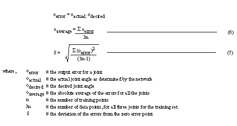
The errors of the solutions were measured in two ways: i) with an average error, and ii) with a deviation [1]. The actual error for a single joint, oerror, is the difference between the actual output, oactual, and the desired output, odesired. The actual error was found for each joint in each training point, and then used as the basis of the subsequent calculations. The average error was found by summing the absolute errors of all the joints for all the training points, and then dividing by the number of training points as seen in equation (6). The deviation was found as in equation (7).

The actual number of training points was 889, thus there were 2667 errors in total. The measure of average error gives a good indication of how close the network is to the ideal solution. The deviation gives an indication of how well grouped the points are. The results from the test runs are available in table 3.

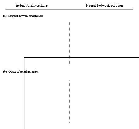
An evenly distributed set of test points, that were not a part of the training set, were presented to the network to evaluate the uniformity of the solutions. Figures 6 displays the topology of the test points for the single plane (i.e. at a constant z level) in this test, z was equal to 0. Please note that the plots are only showing the x, y displacements of the points, but is not showing the z displacement (which is perpendicular to the page). The first plot shows the workspace with the test points evenly distributed. The points in the subsequent cases indicate the neural network’s positioning of the robot arm. The joint coordinates as determined by the neural network where applied to the forward equations to obtain the cartesian locations.

Figure 6 Plot of Inverse Kinematic Distribution

Figure 6(cont’d) Plot of Inverse Kinematic Distribution

In the diagrams, the lines indicate the boundaries of the training region. The points should lie inside and be evenly distributed, as in the first example of figure 6. The discontinuities are obvious on this diagram. The point of the cone is one discontinuity. The circular arc represents the second discontinuity point. The two lines which are along the sides represent the boundaries of the training region only.

Figure 6(cont’d) Plot of Inverse Kinematic Distribution

VIII. Discussion

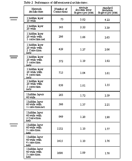
The results in table 3 present a good picture of the relationship between the number of neurons and the generalization capability. When the number of neurons is doubled, the average joint error is reduced by approximately 25%. The standard deviation of the error also decreases by over 20% in the same conditions. The use of correction networks appears to have a beneficial effect upon the network errors. The effect of correction nets was greatest on the networks with fewer neurons. The first three correction networks also tended to have the most effect, but subsequent networks were not very influential.

The points which were well within the training region were placed within a tolerance which was less than one percent of the workspace radius. As the manipulator approaches the discontinuities, the errors become close to 10 percent. The errors increase as the edge of the training region is approached. This suggests that some technique would have to be developed to train the network to deal with, or avoid, the singularities. To correct these problems it may be possible to train the network for the complete volume of the workspace, but not include the regions where singularities occur.

If the singularities are not dealt with, and the network is used as it has been trained here, some problems would be encountered.

Switching from an elbow up to elbow down solution would not be possible, because the network does not approach the singularity very well.

If the quarter of a sphere is mirrored, then a discontinuity is created at intersections of the edges of the training regions. This results because the neural network solution does not perform very well near the edges of the training sphere.

Placing the end of the manipulator over the origin of the robot will result in a singularity configuration.

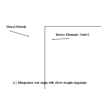
Figure 7 gives a graphic representation of the errors associated when the robot approaches singularity points.

Figure 7 A Comparison of Actual and Neural Network Estimated Position

Figure 7(cont’d) A Comparison of Actual and Neural Network Estimated Position

IX. Conclusions

As the results indicate, this method of robotic control will not be very accurate in certain areas of the workspace; however, the method does work very well when the robot is restricted to small areas in the center of the workspace. These results agree with the work done by Josin [5][6][7]. In his papers, for the planer manipulator, he uses a 2D square in the center of the workspace, to avoid areas of discontinuity. Josin was able to obtain high accuracy by focusing on a subset of the inverse kinematics solution; however, if he were to approach the singularities within his workspace, then his accuracy would decrease. His research was also extended to a 3D wedge volume for the training region with a five link manipulator where the results were highly accurate in this volume. Again, if singular configurations were approached, the generalization capability would surely decrease.

The benefits of the networks are quite distinct. If implemented, the largest inverse kinematics network could be run on a standard Neural Network Accelerator (available for IBM PCs, SUNs, and other computers). Some of the accelerators available run at 10 million connections per second (A few run above 20 million connections per second). This would mean that the network which is 40 neurons wide with 5 correction nets could be processed every 0.17ms or 5900 times per second. For the software which was written for this research, it was possible to process the most complex network in this paper about 150 times per second. The network could have been trained for any manipulator, which indicates that it is a good general technique.

If neural networks are to be implemented as robotic controllers, there are a few points to consider. If a Neural Network controller is trained for a specific manipulator, the network could be saved. When a new controller is attached to a manipulator a pretrained network could be loaded. Sample points may be used for occasional updates to the controller, and thus achieve adaptive control. The ability for such systems to adapt to changes within the environment is an important step towards artificially intelligent machines. In conclusion it must be said that this research must be re-examined when more is understood about Neural Networks.

X. Future Work

Even though the neural networks are not suitable for precise robotic control, they show potential. Neural Networks seem to provide errors similar to what a human would get if the feedback senses were not used for error correction. This suggests that such neural network solutions could be used in a robotic controller that models human flexibility, instead of attempting to obtain superhuman capabilities. This could be done by incorporating a network to estimate inverse kinematics into a feedback system. This system would first estimate the position, determine the error (possibly from a vision system) and then have a second network correct this error. Neural controllers may be applied to autonomous robots such as two-legged "walking" machines where high accuracy is unimportant. If this were to be attempted, then there is indeed a solution to the problem of robot coordination.

Some methods may be researched to help improve the use of neural networks in the inverse kinematics problem. The network could make use of the orientation of the end effector to determine whether an elbow up, elbow down solution or left arm, right arm solution is the best configuration. This network does not provide any estimate of the error. To help detect errors, a neural network model of the forward kinematics could be used to take the inverse kinematic output, and regenerate the x, y, z positions. From this, the error could be used as a confidence measure for the solution.

Neural network solutions are not suited for high precision robotic applications; however, this approach may be useful for generalized robot control such as dynamics, resolved rate control, path planning and task planning. This method could also be used in conjunction with existing methods. If an exact solution is required, and an iterative Inverse Kinematics method must be used, then the neural networks may be used to provide a good initial guess. Another implication of artificial neural networks is the ability to solve previously unknown or intractable problems. Algorithms that require complex computing power for robotic control could be simplified by implementing an artificial neural network controller.

References

[1] Devore, J. L., Probability & Statistics for Engineering and the Sciences. Brooks/Cole Monterey, California, USA, 1982.

[2] Fu, K. S., R. C. Gonzalez, and C. S. G. Lee, Robotics, Control, Sensing, Vision, and Intelligence McGraw-Hill Book Company, New York, NY, USA, 1987.

[3] Guyon, I., Neural Network Systems. Proc. of the INME Symposium, Lausanne, 1989, (to appear).

[4] Guyon, I., I. Poujard, L. Personnaz, G. Dreyfus, J. Denker, Y. LeCun, Comparing Different Neural Architectures for Classifying Handwritten Digits. Proc. of Intern. Jt. Conf. on Neural Networks (IJCNN), Washington, DC, USA, 1989, (to appear).

[5] Josin, G., A Neural Representation of an Unknown Inverse Kinematic Transformation. Proceedings nEuro 88: First European Conference on Neural Networks, Paris, France, June 1988.

[6] Josin, G., Neural-Space Generalization of a Topological Transformation. Biological Cybernetics, vol.59, pp 283: 290, 1988.

[7] Josin, G., D. Charney, and D. White, Robotic Control Using Neural Networks. Proc. of the First European Conference on Neural Networks: nEuro88, 1988.

[8] Lippman, R. P., An Introduction to Computing with Neural Nets. IEEE ASSP Magazine, vol. 4 no. 2, pp 4: 22, April 1987.

[9] Minsky, M. L., and Seymour A. Papert, Perceptrons. MIT Press, 1969.

[10] , Neural Networks. Byte, pp 216: 245, August 1989.

[11] Psaltis, D., A. Sideris, A.Yamamura, Neural Controllers. IEEE First Intern. Conf. on Neural Networks, vol. 4, pp 551: 558, 1987.

[12] Ranky, P. G., and C. Y. Ho, Robot Modelling: Control and Applications with Software.IFS (Publications) Ltd., UK, 1985.

[13] Reber, W. L., and John Lyman, An Artificial Neural System Design For the Rotation and Scale Invariant Pattern Recognition. IEEE First Intern. Conf. on Neural Networks, vol. 4, pp 277: 283, 1987.

[14] Rumelhart, D. E., and James L. McClelland, Parallel Distributed Processing. vol. 1, MIT Press, 1986.

[15] Tourassis, V. D., and Marcelo H. Ang, Jr., A Modular Architecture for Inverse Robot Kinematics. IEEE Trans. on Robotics and Automation, vol. 5, no. 5, pp 555: 568, October 1989.

[16] Wasserman, P. D., Neural Computing: Theory and Practice. Van Nostrand Reinhold, New York, NY, USA, 1988.

Jack, H., Lee, D.M.A., Buchal, R.O., ElMaraghy, W.H., "Evaluations of Neural Networks for Robot Inverse Kinematics", Canadian Society of Mechanical Engineers, 1991.

Abstract