1. EGR 345: Dynamic System Modeling and Control Labs

1.1 Resources

• The following chapters and problems are suggested, in addition to the laboratory materials and the course notes.

• The suggested problems are recommended to help you examine the basic properties of the problems. The required problems must be submitted. Doing only the required problems will leave you at a disadvantage. Historically, students who do not do these problems on a regular basis typically earn final marks that are TWO LETTER GRADES below their peers.

Read Description Suggested

cf 1.1-5 Introduction none

cf 2.1-4 Translation 1,2,4,7,10,12,15,18,22,23,25,27

cf 3.1-3 State Variable Form 3,5,8,9,11,12,13,15,18,21,24,26

cf 4.1-4 Rotation 2,6,7,10,13,18,19,26,29

cf 5.1-7 Electrical systems 3,7,9,12,17,18,21,24,27,31

cf 6.1-6 1st and 2nd order sys. 1,2,5,8,12,16,20,25,27,28

cf 7.1-5 Laplace transforms 3,6a,6b,7,8,10,14,17,21,23,25,32,35

cf 8.1-7 Transfer functions 2,5,7,10,12,14,16,17,20,23,27,29,31,35,39

cf 13.1-5 Block diagrams 1,3,4,6,7,9,13,15,18,24,26,27,30,32,34,36

cf 14.1-5 Feedback and controls 2,5,9,14,17,19,23

1.2 Design Projects

• Overview: This will involve a competitive design to see who can design a servo control system that can respond the fastest.

• Description:

1. The control system will be for a fire-fighting water cannon that has a rotating base. The cannon will actually be a water hose, and the fire will be buckets with marked heights that must be filled. The cannon will start in a neutral position away from the buckets. Once activated the cannon will move to a bucket, fill the bucket, and then move to fill a second bucket. When done the cannon must rotate back to a neutral position.

2. The cannon assembly will be provided, as shown in the figure below. This assembly will include

3. The rules will include a

• Required:

1. A written report describing the design details.

2. A device.

1.3 EGR 345: Laboratory Experiments

• The laboratory work will help enforce the concepts presented in this and previous courses.

• Various labs will require pre- or post-lab work.

• General rules include:

Unless specified, work is to be done individually.

All written work is to be clear and accurate.

• These tutorials prepare you to use computer and other resources throughout the semester.

1.3.1.1 - Tutorial 1a: Creating Web Pages

• The general steps are:

1. Get a computer account on ‘claymore.engineer.gvsu.edu’ from Prof. Jack. This account will have a prototype web page that you can edit.

2. Go to a laboratory (EC 616), or home computer and run ‘Netscape Communicator’. Go to ‘claymore.engineer.gvsu.edu’ and look for your account under ‘students’. You should be able to find a page that starts with ‘YOUR_NAME_GOES_HERE’.

3. In Netscape (with your home page showing), select ‘edit’ from the tool bar, or under ‘file’ select ‘edit’ or ‘edit page’. You will be asked if you want to save the page. Create a ‘temp’ directory on the computer. This directory will be used to temporarily hold your web page files. Make sure that the files will be saved in the ‘temp’ directory, and then ‘save’ the files. An editor will start on the screen.

5. The editor behaves much like Microsoft Word, with some subtle differences. At this point add your name, and change your email address to your river account. You can change your email address by clicking on the email link, and then clicking on the chain link near the top of the screen.

6. To upload the changes you have made to the website, select ‘publish’. You will need to indicate the file name as ‘index.html’, the destination as ‘ftp://claymore.engineer.gvsu.edu/home/YOUR_NAME/public_html’. You will also need to enter your user name and your password (DO NOT SAVE THE PASSWORD: SOMEBODY ELSE CAN GET ACCESS TO YOUR ACCOUNT). You should see a message that indicates files have been uploaded successfully.

7. Use Netscape, not the editor, to see if the changes have occurred. Your changes may not show up on the browser. This is because Netscape does not reload pages every time to look at them. Pages are often stored for up to 1 month on the PCs hard drive, and reused when you look at them. There are two ways to update the screen before this time limit: click on the reload button.

8. Next we will add links to your home page. First, run Mathcad, and create a simple file, and then save it in the same folder/directory you saved. Use a file name that is all lower case such as ‘test.mcd’: any upper case letters cause problems in Windows 95.

9. Get your home page back in the Netscape editor. Someplace type the word ‘GVSU’. Use the mouse to select what you just typed, and then click on the link button. For the link name enter ‘http://www.gvsu.edu’, and apply the change. This will now be a link to the Grand Valley home page. For your Mathcad file type something like ‘Mathcad file’, highlight it, and add a link to ‘test.mcd’. This link will connect to your Mathcad file.

10. Publish the file, but first add the Mathcad file to the list of files at the bottom of the screen.

11. Test the page.

• Some tips are,

Windows will not allow multiple applications to open the same file at the same time. If you seem to be having trouble opening a file, make sure it is not open in another application.

As you add other files to your homepage, put them in the ‘temp’ directory. This will make all of the procedures simpler.

Try to make your web pages small, and link them together. This will decrease download time and make browsers happier.

Avoid using excessive images. Anything over 10K will make it very slow downloading over modem. Anything over 100K makes modem downloading painfully slow.

When putting images on the web page use ‘jpg’ for photographic images, and ‘gif’ for line images. ‘jpg’ images can be compressed more than ‘gif’, but lines will become blurred.

To link to other files or web pages there will be a ‘link’ command. If you want to add a file that is in your ‘temp’ directory, just put the name of the file in the ‘URL’ field.

Watch upper/lower case. This is a major cause of web page problems. It is best to keep to lower case for all file names.

1.3.1.2 - Tutorial 1b: Introduction to Mathcad, Working Model 2D and The Internet

• Objective:

Working Model 2D, Mathcad and the Internet will be used in this course. In some cases students have not been exposed to one or more of these software packages in the past. This session will be used as a refresher for those with little prior exposure, and as a tutorial for those with no experience.

• Theory:

Mathcad is a software package that allows us to do complex calculations both numerically and symbolically. To learn it initially will require a time investment. But, when doing calculations later, it will save a significant amount of time and reduce calculation errors.

Working Model 2D is a software package that allows us to set up systems of multiple rigid bodies. We can then apply forces, moments, etc. and then see how the system dynamics are effected. In comparison, Mathcad will allow longer, precise calculations, whereas Working Model allows faster results with reduced accuracy. Working Model also presents a visual simulation: this allows a more intuitive understanding of a dynamic system.

The Internet is a huge collection of computers providing information and connection on an unprecedented scale. It has become a standard business tool, and continues to evolve.

• Procedure

1. (If needed) Go over the Mathcad tutorial provided.

2. Use Mathcad to calculate the position of a ball that has been held then released just above the surface of the earth, and add the file to your home page.

3. (If needed) Go over the Working Model tutorial provided.

4. Repeat the problem solved in Mathcad with Working Model and add the file to your home page.

5. (If needed) Get a computer account set up, and create a home page.

6. Go to a search engine and find a website for a major business that is related to your co-op position and add a link to it on your home page. Explain how the business is related to your co-op position.

• Post-lab:

None

• Submit:

1. A Mathcad file linked to your home page.

2. A Working Model file linked to your home page.

3. An explanation and a link to a company on your home page.

1.3.1.3 - Presentation 1a: Introduction to Library Searches

• Objective:

To prepare students to use the libraries resources in typical research studies.

• Theory:

The essential purpose of engineering is to apply principles of the arts and sciences to solve real problems. Scientific principles tend to evolve over time, but the essential principles and written works are valid for a number of decades or centuries. As a result, books can be excellent resources for this knowledge. The applications that make use of the basic principles tend to be more revolutionary. As a result, printed books have a value for teaching the fundamentals, but the ’state of the art’ must often be found in magazines, journals, etc. To put this in simpler terms, when we look for scientific resources, we will often use sources over a decade old. When using engineering resources, most will be less than five years old. Until recently, print has been the major means of exchanging information, and libraries have been the traditional repositories of printed materials. To deal with the extensive number of publications available in a library, we need to learn how to search for needed information, and what resources are available.

New technology has changed access to library materials. Libraries pool resources and share materials. Internet technology has also helped increase accessibility. In particular internet tools allow the entire library catalog to be examined without visiting the library. There are also a number of resources that can be searched and retrieved over the internet.

• Procedure

1. A presentation will be made by Mr. Lee Lebin, the University Library Director.

2. Use the library resources to identify an application of systems modeling.

• Post-lab:

1. Search for library resource.

• Submit:

1. A copy of the material referenced.

1.3.2.1 - Prelab 2a: Tutorial for LabVIEW Programming

Objective:

To learn the basic use of LabVIEW.

Theory:

To obtain the greatest computing power and flexibility we need to write computer programs. But, traditional programming languages are not well suited to designing user interfaces and dealing with data flows.

Most computer programs are written with lines of program and compiled to execute. LabVIEW allows you to “write” programs using graphical symbols. This graphical programming approach allows systems to be designed by connecting the symbols with "wires" (i.e., lines).

Equipment:

PC with LabVIEW software

Procedure:

1. Go through the LabVIEW QuickStart Guide provided in the laboratory. This will also be good review for those who have used LabVIEW in previous courses.

2. Write a Labview program that will count from 1 to 100, square the values, and print the results on a strip chart.

Marking:

1. The VI created should be posted to the web.

1.3.2.2 - Prelab 2b: Overview of Labview and the DAQ Cards

• To obtain the greatest computing power and flexibility we need to write computer programs. But, traditional programming languages are not well suited to designing user interfaces and dealing with data flows.

• LabVIEW allows you to “write” programs using graphical symbols. This graphical programming approach allows systems to be designed by connecting the symbols with "wires" (i.e., lines).

• The remainder of the labs will focus on using LabVIEW to write programs to allow a computer to interact with the environment outside the computer.

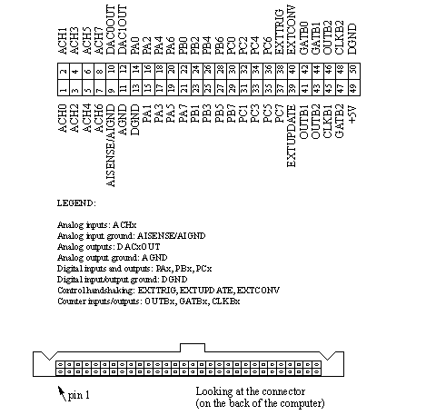
• The computers we will use all have DAQ (Data AcQuisition) boards: National Instruments PCI-1200 DAQ cards. These cards have capabilities that include:

24 I/O bits: TTL 0,5VDC, 20mA max.

8 single ended or 4 double ended analog inputs: 12 bits

3 counters: 16 bits

2 analog outputs: 12 bits

• The connector for the card can be found on the back of the computer. It will have a connector with pinouts like the one shown below. A ribbon cable will be used to make electrical connection to the connector in the back of the computer.

 

NOTE: LABVIEW MANUALS ARE AVAILABLE ON-LINE, AND CAN BE FOUND ON THE COURSE HOME PAGE: LEAVE THE PAPER MANUALS IN THE LAB.

1.3.2.3 - Experiment 2: Introduction to LabVIEW and the DAQ Cards

Objective:

Learn to use computers equipped for A/D and digital inputs.

Theory:

The computer reads data at discrete points in time (like a strobe light). We can read the data into the computer and then do calculations with it.

To read the data into a computer we write programs, and use "canned" software to help with the task. LabVIEW allows us to write programs for data collection, but instead of typing instructions we draw function blocks and connect them. How we connect them determines how the data (numbers) flow. The functions are things like data reads and calculations.

In this lab we will be using Labview to connect to a data acquisition (DAQ) board in the computer. This will allow us to collect data from the world outside the computer, and make changes to the world outside with outputs.

When interfacing to the card using a program such as Labview, there must be ways to address or request information for a specific input or output (recall memory addresses in EGR226). The first important piece of information is the board number. There can be multiple DAQ boards installed in the computer. In our case there is only one, and it is designated device ’1’. There are also many inputs and outputs available on the card. For analog outputs there are two channels so we need to specify which one when using the output with 0 or 1. For analog inputs there are 8 channels, and as before, we must specify which one we plan to read from using 0 to 7. For digital I/O there are a total of 24 pin distributed across 3 ports (1 byte each). Therefore when connecting inputs and output we must specify the port (PA=0, PB=1, PC=2) and the channel from 0 to 7. Note is that we can make the ports inputs or outputs, but not mixed: in other words we must pick whether a port will only be used for inputs or for outputs.

The voltage levels for the inputs and outputs are important, and you will need to be aware of these. For the digital outputs they will only ever be 0V or 5V. But the analog inputs and outputs will vary from -5V to 5V. This is build into the board. If we exceed these voltage limits by a few volts on the inputs, the boards have built in protection and should be undamaged. If we exceed the input voltages significantly, there is a potential to permanently damage the board.

Equipment:

PC with LabVIEW software and PCI-1200 DAQ card

Interface cable

PLC trainer boards

Signal generator

Digital multimeter

Procedure:

1. Go through the LabVIEW QuickStart Guide provided in the laboratory. This will also be good review for those who have used LabVIEW in previous courses.

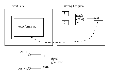
2. Enter the LabVIEW program (layout) schematically shown below and connect a signal generator to the analog input (ACH0). (Note: there is a pin diagram for the connector in the Labview tutorial section.) Start the signal generator with a low frequency sinusoidal wave. Use the ‘DAQ Configure’ software to test the circuitry and verify that your hardware is operational. Then run your Labview program. Record the observations seen on the screen.

 

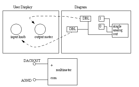
3. Connect the multimeter as shown below. Test the circuit using the ‘DAQ Configure’ utility. Enter the LabVIEW program schematically illustrated below and then run it. You should be able to control the output voltage from the screen using the mouse. Record your observations.

 

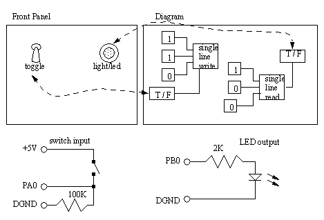
4. Connect the digital input and output circuits to the DAQ card and use the test panel to test the circuits. To do this, run the ‘DAQ Configure’ utility, double click on the ‘PCI-1200’, run the test panel window and ensure that the inputs and outputs are working correctly. Create the LabVIEW screen schematically illustrated below. This should allow you to scan an input switch and set an output light. When done, quit the program and run your LabVIEW program.

 

Marking:

1. A laboratory report should be written, including observations, and posted to the web.

2. The programs (VIs) that use the DAQ card should be posted to the web.

1.3.3.1 - Prelab 3: Sensors

Theory:

Sensors allow us to convert physical phenomenon to measurable signals, normally voltage or current. These tend to fall into one of two categories, discrete or continuous. Discrete sensors will only switch on or off. Examples of these include,

Inductive Proximity Sensors: use magnetic fields to detect presence of metals

Capacitive Proximity Sensors: use capacitance to detect most objects

Optical Proximity Sensors: use light to detect presence

Contact Switches: require physical contact

Continuous sensors output values over a range. Examples of these are,

Potentiometers: provide a resistance proportional to an angle or displacement

Ultrasonic range sensors: provides a voltage output proportional to distance

Strain Gages: their resistance changes as they are stretched

Accelerometers: output a voltage proportional to acceleration

Thermocouples: output small voltages proportional to temperature

In both cases these sensors will have ranges of operation, maximum/minimum resolutions and sensitivities.

Prelab:

1. Prepare a Mathcad sheet to relate sensor outputs to the physical phenomenon they are measuring.

1.3.3.2 - Experiment 3: Measurement of Sensor Properties

Objective:

To investigate popular industrial and laboratory sensors.

Procedure:

1. Sensors will be set up in the laboratory at multiple stations. You and your team should circulate to each station and collect results as needed. Instructions will be provided at each station to clarify the setup. The stations might include,

a mass on a spring will be made to oscillate. The mass will be observe by measuring position and acceleration.

a signal generator with an oscilloscope to read voltages phenomenon observe should include sampling rates and clipping.

2. Enter the data into Mathcad and develop a graph for each of the sensors relating input and output.

Submit:

1. A full laboratory report with graphs and mathematical functions for each sensor.

1.3.3.3 - Experiment 3b: Brushless Servo Motors and Controls

Objective:

To investigate industrial motors and controllers and develop a mathematical model.

Theory: The industrial motors and controllers to be used in this laboratory are manufactured by Allen-Bradley. The controllers are Ultra 100 drives, and the motors are Y-series brushless servo motors.

Prelab:

1. Visit the Allen Bradley web site (www.ab.com) and investigate the controllers and mototrs to be used in this laboratory: Ultra 100 drives and Y-1003-2H motors.

Procedure:

1. Follow the provided tutorial for Ultra 100 drives.

Submit:

1. Graphs of response curves

2. A mathematical model of ______

• This set of labs will examine devices that have multiple phenomenon occurring.

1.3.4.1 - Prelab 4a: Permanent Magnet DC Motors

• Theory:

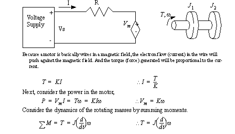
DC motors will apply a torque between the rotor and stator that is related to the applied voltage or current. When a voltage is applied the torque will cause the rotor to accelerate. For any voltage and load on the motor there will tend to be a final angular velocity due to friction and drag in the motor. And, for a given voltage the ratio between steady state torque and speed will be a straight line.

 

The basic equivalent circuit model for the motor is shown below. We can develop equations for this model. This model must also include the rotational inertia of the rotor and any attached loads. On the left hand side is the resistance of the motor and the ’back emf’ dependent voltage source. On the right hand side the inertia components are shown. The rotational inertia J1 is the motor rotor, and the second inertia is an attached disk.

 

The model can now be considered as a complete system.

 

Looking at this relationship we see a basic first order differential equation. We can measure motor properties using some basic measurements.

• Prelab:

1. Integrate the differential equation to find an explicit function of speed as a function of time.

2. Develop a Mathcad document that will accept values for time constant, supplied voltage and steady state speed and calculate the coefficients in the differential equation for the motor.

3. In the same Mathcad sheet add a calculation that will accept the motor resistance and calculate values for K and J.

4. Also add a calculation to use the unloaded motor torque the motor is stalled (omega = 0) to find the K value.

5. Get the data sheets for an LM675 from the web (www.national.com).

1.3.4.2 - Experiment 4a: Modeling of a DC Motor

• Objective:

To investigate a permanent magnet DC motor with the intention of determining a descriptive equation.

• Procedure

1. With the motor disconnected from all other parts of the circuit, measure the resistance across the motor terminals.

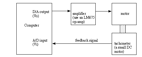
2. Connect the motor amplifier, motor and computer as shown in the figure below.

 

3. Write a Labview program that will output an analog output will be used to drive the motor amplifier. An analog input will be used to measure the motor speed from the tachometer.

4. Use a strobe light to find the relationship between the tachometer voltage and the angular speed.

5. Obtain velocity curves for the motor with different voltage step functions.

6. Use a fish scale and a lever arm to determine the torque when the motor is stalled with an input voltage.

• Post-lab:

1. Determine the values of K for the motor. Determine the J for the rotor, and calculate J values for different load masses added.

2. Use the values of R, J and K to compare theoretical to the actual motor response curves found in procedure step #5.

3. Use the values of R, J and K to determine what the stalled torque should be in procedure step #6. Compare this to the actual.

4. Find the time constant of the unloaded motor.

• Submit:

1. All work and results.

1.3.5.1 - Prelab 5a: DC Servo Motor PID Controller

• Theory:

 

Recall that by itself a motor is a first order system, but by adding a mass to it will become a second order system. A PID controller is well suited to controlling second order systems. But, tuning a PID controller is an art. The proportional gain sets to overall response. This should be tuned first so that the motor generally responds quickly, but doesn’t overshoot the goal. The derivative term should be set next so that the motor responds faster, and only overshoots the goal by an acceptable amount. Finally the integral portion is used to reduce the steady state error.

• Prelab:

1. Try the PID controller example in Labview.

2. Review the course notes on the PID controller.

3. Set up a Mathcad sheet to store/calculate rise time, settling time, overshoot, damping ratio, natural frequency.

1.3.5.2 - Experiment 5a: DC Servo Motor PID Controller

• Objective:

To investigate a simple motor controller.

• Procedure

1. Set up the feedback controller for PID control, and test for basic operation.

2. Vary the time constants and gain, and record the responses to an input step function. Calculate the important parameters, such as damping ratio and natural frequency.

3. Tune the controller for the best response (i.e. damping ratio = 1) using the technique described in the theory section.

• Post-lab:

1. Compare the final PID values with the simulated response for the system.

• Submit:

1. All work.

• DC motors are common system components to drive mechanical systems.

• Understanding how these motors behave is important.

1.3.6.1 - Prelab 6a: Servomotor Proportional Control Systems

• Theory:

DC servomotors typically have a first order (velocity) response as found in a previous lab.

 

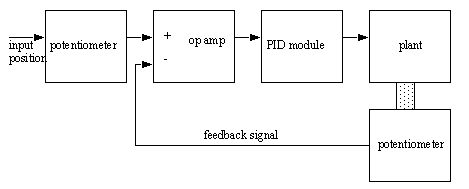
We can develop a simple control technique for control of the velocity using the equation below. For this form of control, we need to specify a desired velocity (or position) by setting a value ’Vd’. The difference between the desired speed and actual speed is calculated (Vd-Vi). This will give a voltage difference between the two values. This difference is multiplied by a constant ’K’. The value of ’K’ will determine how the system responds.

 

The basic controller is set up as shown in the figure below. We can use a Labview program to implement the basic control equation described above.

 

• Prelab:

1. Develop a Mathcad document that will model the velocity feedback controller given, motor parameters, desired velocity, an inertial load, and a gain constant. This is to be solved three different ways i) with Runge-Kutta integration, ii) integration of differential equations and iii) with laplace transforms.

2. Test the controller model using a step function.

3. Repeat steps 1 and 2 for a position controller system.

1.3.6.2 - Experiment 6a: Servomotor Proportional Control Systems

• Objective:

To investigate simple proportional servo motor control.

• Procedure

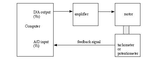
1. Set up the same system used for measuring the motor velocity in the previous lab. This will be a velocity control system. Apply a step function input and record the response.

2. For several values of proportional gain ’K’, measure the response curves of the motor to a step function.

3. Replace the tachometer with a potentiometer, and repeat steps 1 and 2.

• Post-lab:

1. Compare the theoretical and actual response curves on the same graphs.

2. Find and compare the time constants for experimental and theoretical results.

• Submit:

1. All work and results.

1.3.7.1 - Prelab 7a: Mechanical Components

• Theory:

Recall that for a rigid body we can sum forces. If the body is static (not moving), these forces and moments are equal to zero. If there is motion/acceleration, we use d’Alembert’s equations for linear motion and rotation.

 

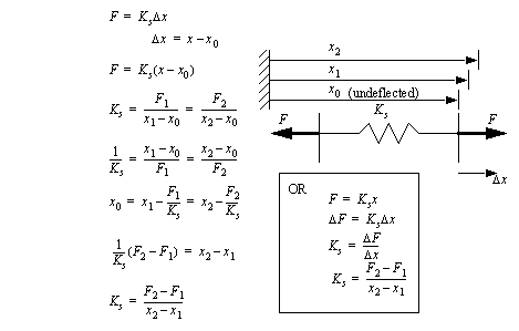
If we have a system that is comprised of a spring connected to a mass, it will oscillate. If the system also has a damper, it will tend to return to rest (static) as the damper dissipates energy. Recall that springs ideally follow Hooke’s law. We can find the value of the spring constant by stretching the spring and measuring the forces at different points or we can apply forces and measure the displacements.

 

In many cases we will get springs and devices that are preloaded. Both of the devices used in this lab have a preloaded spring. This means that when the spring has no force applied and appears to be undeflected, it is already under tension or compression, and we cannot use the unloaded length as the undeflected length. But, we can find the true undeflected length using the relationships from before.

 

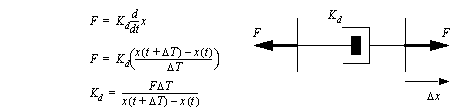
Next, recall that the resistance force of a damper is proportional to velocity. Consider that when velocity is zero, the force is zero. As the speed increases, so does the force. We can measure this using the approximate derivatives as before.

 

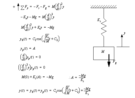
Now, consider the basic mass-spring combinations. If the applied forces are static, the mass and spring will remain still, but if some unbalanced force is applied, they will oscillate.

 

 

In the lab an ultrasonic sensor will be used to measure the distances to the components as they move. The sensor used is an Allen Bradley 873C Ultrasonic Proximity Sensor. It emits sound pulses at 200KHz and waits for the echo from an object that is 30 to 100cm from it. It outputs an analog voltage that is proportional to distance. This sensor requires a 18-30 VDC supply to operate. The positive supply voltage is connected to the Brown wire, and the common is connected to the blue wire. The analog voltage output (for distance) is the black wire. The black wire and common can be connected to a computer with a DAQ card to read and record voltages. The sound from the sensor travels outwards in an 8 degree cone. A solid target will give the best reflection.

• Prelab:

1. Review the theory section.

2. Extend the theory by finding the response for a mass-spring, mass-damper, and mass-spring-damper system (assume values).

3. Set up a Mathcad sheet for the laboratory steps.

1.3.7.2 - Experiment 7a: Mechanical Components

• Objective:

This lab will explore a simple translational system consisting of a spring mass and damper using instrumentation and Labview.

• Procedure

1. Use two masses to find the spring constant or stiffness of the spring. Use a measurement with a third mass to verify. If the spring is pretensioned determined the ’undeformed length’.

2. Hang a mass from the spring and determine the frequency of oscillation. Determine if the release height changes the frequency. Hint: count the cycles over a period of time.

3. Connect the computer to the ultrasonic sensor (an Allen Bradley Bulletin 873C Ultrasonic Proximity Sensor, see www.ab.com), and calibrate the voltages to the position of the target (DO NOT FORGET TO DO THIS). Write a Labview program to read the voltage values and save them to a data file. In the program set a time step for the voltage readings, or measure the relationship between the reading number and actual time for later calculation.

4. Attach a mass to the damper only and use Labview to collect position as a function of time as the mass drops. This can be used to find the damping coefficient.

5. Place the spring inside the damper and secure the damper. This will now be used as a combined spring damper. In this arrangement the spring will be precompressed. Make sure you know how much the spring has been compressed when the damper is in neutral position.

6. Use the spring-damper cylinder with an attached mass and measure the position of the mass as a function of time.

7. Use Working Model 2D to model the spring, damper and spring-damper responses.

• Post-lab:

1. Determine if the frequency of oscillation measured matches theory.

2. Compare the Labview data to the theoretical data for steps 2, 4 and 6.

3. Compare the Labview data to the working model simulations.

• Submit:

1. All results and calculations posted to a web page as a laboratory report.

• Many systems undergo periodic motion. For example, the pendulum of a clock.

• To observe high frequency oscillations we need high speed data collection devices. The LabVIEW applications you have previously created are no longer adequate.

• To collect data faster we now will use an oscilloscope interfaced to LabVIEW.

1.3.8.1 - Prelab 8a: Oscillating Systems

• Theory:

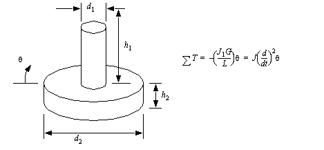
Suppose a large symmetric rotating mass has a rotational inertia J, and a twisting rod has a torsional spring coefficient K. Recall the basic torsional relationships.

 

We can calculate the torsional spring coefficient using the basic mechanics of materials

 

Finally, consider the rotating mass on the end of a torsional rod.

 

• Prelab:

1. Calculate the equation for the natural frequency for a rotating mass with a torsional spring.

2. Set up a Mathcad sheet that will

accept material properties and a diameter of a round shaft and determine the spring coefficient.

accept geometry for a rectangular mass and calculate the polar moment of inertia.

use the spring coefficient and polar moment of inertia to estimate the natural frequency.

use previous values to estimate the oscillations using Runge-Kutta.

plot the function derived using the homogeneous and particular solutions.

1.3.8.2 - Experiment 8a: Oscillation of a Torsional Spring

• Objective:

To study torsional oscillation using Labview and computer data collection.

• Procedure

1. Calibrate the potentiometer so that the relationship between and output voltage and angle is known. Plot this on a graph and verify that it is linear before connecting it to the mass.

2. Set up the apparatus and connect the potentiometer to the mass. Apply a static torque and measure the deflected position.

3. Apply a torque to offset the mass, and release it so that it oscillates. Estimate the natural frequency by counting cycles over a long period of time.

4. Set up LabVIEW to measure the angular position of the large mass. The angular position of the mass will be measured with a potentiometer.

• Post-lab:

1. Compare the theoretical and experimental values.

• Submit:

1. All work and observations.

2. Post the laboratory report to a web page.

1.3.9.1 - Prelab 9: Filtering of Audio Signals

Theory:

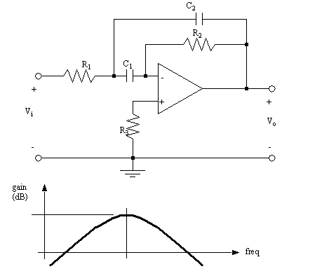
We can build simple filters using op-amps, and off the shelf components such as resistors and capacitors. The figure below shows a band pass filter. This filter will pass frequencies near a central frequency determined by the resistor and capacitor values. By changing the values we can change the overall gain of the amplifier, or the tuned frequency.

 

The equations for this filter can be derived with the node voltage method, and the final transfer function is shown below.

 

 

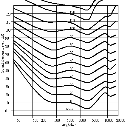
As dictated by the ear, audio signals have frequencies that are between 10Hz and 16KHz as illustrated in the graph below. This graph shows perceived sound level, with the units of ’phons’. For example, we can follow the 100 phons curve (this would be like a loud concert or very noisy factory requiring ear protection). At much lower and higher frequencies there would have to be more sound pressure for us to perceive the same loudness, or phon value. If the sound were at 50Hz and 113 dB it would sound as loud as 100dB sound at 1KHz.

 

You may appreciate that these curves are similar to transfer functions, but they are non-linear. For this lab it is important to know how the ear works because you will be using your ear as one of the experimental devices today.

Prelab:

1. Derive the transfer function given in the theory section.

2. Draw the Bode plot for the circuit given R1=R2=1000ohms and C1=C2=0.1uF. You are best advised to use Mathcad to do this.

1.3.9.2 - Experiment 9: Filtering of Audio Signals

Objective:

To build and test a filter for an audio system.

Procedure:

1. Set up the circuit shown in the theory section. Connect a small speaker to the output of the amplifier.

2. Apply a sinusoidal input from a variable frequency source. Use an oscilloscope to compare the amplitudes and the phase difference. Also record the relative volumes you notice.

3. Supply an audio signal, from a radio, CD player, etc. Record your observations about the sound.

Submit:

1. Bode plots for both theory and actual grain and phase angle.

2. A discussion of the sound levels you perceived.

1.4 Tutorial - Ultra 100 Motors and Drives

1. Obtain the motor and controller sets. This should include a brushless servo motor (Y-1003-2H), an Ultra 100 Controller and miscellaneous cables. The cables are described below. located and verify they are connected as indicated in the sequence given below.

a) the motor is connected to the controller with two cables, one for the power to drive the motor, and the other a feedback from the encoder. The encoder is used to measure the position and velocity of the motor. If not connected already, connect these to the motor controller.

b) the controller should also have a serial cable for connecting to a PC serial port. Connect this to a PC.

c) a custom made connector will be provided with some labelled wires. This will be used to connect to other devices for experimental purposes.

d) a power cord to be connected to a normal 120Vac power source. DO NOT CONNECT THIS YET.

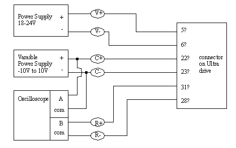
2. The custom made connector needs to be attached to devices to control and monitor the motor. The figure below shows a test configuration to be used for the tutorial. The letters in ovals correlate to the ends of the provided connectors. Do not turn on the devices yet.

 

3. Plug in the power cord for the Ultra 100 drive and look for a light on the front to indicate that it is working. WARNING: The motor might begin to turn at this point. Turn on the power supplies and the oscilloscope.

4. Run the ’Ultramaster’ software on the PC. When prompted select ’drive 0’. At this point the software should find the drive and automatically load the controller parameters from the controller. when it is done a setup window will appear.

5. In the setup window ensure the following settings are made. When done close the setup window.

Motor Type: Y-1003-2-H: this is needed so that the proper electrical and mechanical properties of the motor will be used in the control of the motor (including rotor inertia).

Operation Mode Override: Analog Velocity Input: This will allow the voltage input (C+ and C-) to control motor velocity.

6. Select the ’Drive Configuration’ window and make the following settings.

Analog Output 1: Velocity: Motor Feedback: this will make the analog voltage output from the controller (R+ and R-) indicate the velocity of the motor, as measured by the encoder.

Scale: 500 RPM/VOLT: this will set the output voltage so that every 500RPM will produce an increase of 1V.

7. Open the Oscilloscope on the computer screen and make the following settings. When done position the oscilloscope to the side of the window so that it can be seen later.

Channel A: Velocity: command

Channel B: Velocity: motor feedback

Time Base: 50ms

8. Open the control panel and change the speed with the slider, or by typing it in. Observe the corresponding changes on the oscilloscope on the screen, and the actual oscilloscope.

9. Hold the motor shaft while it is turning slowly and notice the response on the oscilloscopes.

10. Open the tuning window and change the ’I’ value to 0. Change the motor speed again and notice the final error. It should be larger than in previous trials.

11. Leave the ’I’ value at ’0’ and change the ’P’ value to 50 and then change the speed again. This time the error should be larger, and the response to the change should be slower.

12. Try other motor parameters and see how the motor behaves. Note that very small or large values of the parameters may lead to controller faults: if this occurs set more reasonable ’P’ or ’I’ values and then reset the fault.

13. Set the parameters back to ’P’ = 200 and ’I’ = 66.

14. Stop the ’Control Panel’, this will allow the motor to be controlled by the external voltage supply. Change the voltage supply and notice how the motor responds.

ADD: POSITION CONTROL, TORQUE CONTROL, CHANGING MOTION PROFILE

1.5 Tutorial - Labview Based IMAQ Vision

1. Locate the appropriate hardware and software for the laboratory. This includes a video camera with an appropriate lens attached. A BNC cable to connect to the computer. A computer with the National Instruments IMAQ PCI-1408 vision card and IMAQ software installed.

2. We will start by verifying that the vision system is working properly. To do this run the “IMAQ Configuration Utility”. You should see a screen that shows the computer and PCI-1408 card. Click on the ‘+’ to the left of the card and you should see four input channels appear. The first of these is ‘channel 0’, click on it. Next, select “Aquire”, “Grab”, a window should appear that shows a video feed. Adjust/focus the lens until a clear image appears. Note that the lens attached is a TV lens. For small distances (less than 2-3 feet) the lens will be very sensitive to focus, when a longer focus is used it will be much less sensitive. Explore the software settings for the camera. Feel free to change values, but record the original value so that it may be changed back. When you feel comfortable that the video images are being captured properly, continue to the next step.

3. Run Labview, and open a “New vi”. Construct the vi below to capture an image and display it on the screen.

 

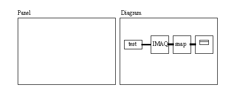
(From left to right) First create a string, and enter ‘test’ or something else. Next create the ‘IMAQ’ icon using “IMAQ Vision”, “Management”, “IMAQ”. This will create a generic place to store images. At this point the image size, etc is not important. Now that we have a place to store the image, we can grab images from the camera with the ‘snap’ icon found at “Image Aquisition”, “Snap”. Finally we can display the images using the last icon found at “IMAQ Vision”, “Display (basics)”, “IMAQ WindDraw”. Connect these together and run the vi. You should see an image from the camera. Notice that these icons are doing a lot that is not on the screen. The vision add-on to Labview does not fully follow the philosophy of graphical programming. Things like the display window are not shown in the panel where they should be. These ‘cheats’ are necessary because of the huge amount of data required for vision tasks. Take some time to explore the other vision tools, and try modifying the vision program.

4. Close the vi and do not save changes to any other vi (this could save some settings permanantly). Next, use “Open vi” and open “examples”, “vision”, “barcodedemo.vi”. Run the vi. An image of a barcode should appear. Use the mouse to put a rectangle over the bar code. Then accept the Region of Interest “ROI”. After this the program will use images saved on disk to test the routine. The codes should match the displayed images. Stop the vi and look at the diagram to see the general operation: it is set up to use a sequence. Notice that the first frame in the sequence pulls an image from a file, and displays it on the screen. The next couple of frames deal with getting the region of interest. The fourth sequence (3 of 0 to 4) captures images and decodes the barcodes. The last sequence is used to release the vision memory, etc. Notice that the images are being supplied by a function called “simu GRAB”, replace this with the normal snap routine and run the program (put a vi in front of the camera). You should now see the images, but they are not decoded properly. Notice that the barcode icon has an integer digit input of ‘3’, you will need to change this value to get the barcodes to decode properly.

5. Close the vi (don’t save any changes). Open the example vi “caliperdemo.vi”, and run the vi. This vi can be used to check the presence of objects. Draw lines across the image. Each point where the line goes from light/dark or dark/light an edge will be detected. If the line is accepted you will see it appear on the list, you will want to change the number of edges. You can have more than one test line. When done run the test and see how it behaves. Look at the diagram for the vi and modify it to use the camera (as you did for the barcode reader).

1.6 Lab - Vision Systems for Inspection

Purpose:

A vision system will be explored and implemented in the laboratory setting.

Overview:

The vision system is based on Labview. A dedicate PC will be used in the cell to process the vision commands. Using labview the PC can then be connected to the Soft PLC controller.

Pre-Lab:

1. Review labview programming using tutorials found at the national instruments site (www.natinst.com).

In-Lab:

1. Complete the Labview vision tutorial.

2. Modify the appropriate test program to read bar codes, and save them to a file

3. Modify the appropriate test program to read a dimension of arbitrary parts and write the dimension to a serial port.

Submit:

1. Printouts of the modified test programs.

1.7 Tutorial - DVT Cameras

(******To be done outside the lab without the hardware)

1. If the DVT software is not installed yet, install it now.

2. In either case put the DVT CDRom in the computer and follow the tutorials on the CD.

3. Run the ’Framework’ software. When it starts to run a window called ’PC Communications’ will appear. In this case we will only use the simulator, so select ’Emulator’ then ’Model 630’, then ’Connect’. The emulator will also start as another program.

4. At this point we can set up a simple set of vision tests for the camera. The camera is capable of supporting tests for more than one product. You can select which product the tests will be for by first selecting ’Products’ then ’Product Management...’. This will put up a window to define the product details. Select ’New’ and then enter ’part1’. Use ’OK’ to dismiss the windows and get back to the main programming window.

5. We need to now set up the emulator to feed images to the programming software. We can do this by loading a set of test images. To do this open the ’DVT SmartImage Sensor Emulator’ window. Then select ’Configure’ then ’Image sequence...’. Select ’Browse for Image’ and then look for images on the CD in the ’emulator\images\Measurement’ directory. Pick the file ’Measurement001.bmp’. The next window will ask for the last image so select ’Measurement010.bmp’. Select ’OK’ to get back to the main emulator window.

6. Go back to the Framework programming screen. The emulator can be started by selecting the right pointing black triangle near the red circle. You should see images appear in a sequence. Pause the images using the single vertical line.

7. Next we will add a test to the product. On the left hand side of the screen select ’Measurement’, select the small line with two red arrows and then move the mouse over the picture and draw a line over a single section of the part, for example the right hand most side by the large circle.

8. In the pop-up window enter the test name ’test1’. Apply the changes and dismiss the window and run the camera again. Notice that as the images flip by the result of the test is shown at the bottom of the screen. As the images are captured the part may move around. It is common to delete and recreate the sensor a number of times to find the right position for the line. Double click on the sensor and look at some of the options possible. Try changing these and see what happens.

9. Delete the previous sensor and create a sensor (rotational positioning: find edge in parallelogram), and a translation sensor (translational positioning: fudicial rectangle). For the translation sensor, under the ’Threshold’ select ’Dark Fudicial’. Run the software and note the rotation and translation data at the bottom of the screen as the images are processed.

10. Delete the sensors. Go to the emulator and load the two ’1dBarCode’ images in the ’emulator\images\1DReader’. In Framework run the camera so that these appear on the screen, then pause the camera. On the left hand side of the screen select ’Readers’ then ’Barcode Sensor: Line for 1D codes’. Draw the sensor line over the middle of the barcode.

1.8 Lab - Vision Systems for Inspection

Purpose: To learn to use the DVT cameras as input sensors for PLCs

Overview: The DVT cameras are selfcontained vision systems. At the simplest these process images and perform checks that result in pass fail test results.

Pre-Lab:

1. Follow the tutorial for the DVT units.

2. Review the manual for the 630 camera at www.dvtsensors.com

3. Develop a system as suggested in the process below. This should include at least wiring diagrams and ladder logic.

Process:

The process will have a motor that drives a conveyor system. As parts move along the belt they are detected with a proximity sensor. When they move into range of the sensor the camera should perform a test for quality control. If the part is to be rejected a cylinder will fire and eject the part.

In-Lab:

1. Follow the DVT quickstart book to become familiar with the hardware.

2. Build the system designed in the prelab and select a ’part’ to test it with.

1.9 CNC Machining

Purpose:

The students will be introduced to the basics of CNC equipment.

Overview:

A simple tutorial will be used to introduce the students to the CNC equipment in the laboratory. The students will develop a simple G-code program to cut their initials on the mill and a candle stick on the lathe. Both programs can be simulated off-line, and then tested in the laboratory. You will also be introduced to automatic part programming software.

Pre-Lab:

1. Review the course material on CNC machines, and specifics for the PC-turn 50, and Pro-light machines.

2. Use netscape to explore the NC machines in the laboratory.

3. Develop by hand a program to cut your initials using the Pro-light NC mill. The initials will be cut on a 2” square piece of aluminum. Correct speeds and feed should have also been determined.

4. Develop by hand a program to cut a candlestick in brass with a 1” dia on the PC-turn 50 lathe. Correct speeds and feed should have also been determined.

5. Simulate both programs before arriving at the laboratory.

In-Lab:

1. In the lab you will be shown how to set up the NC lathe and mill, fixture parts, and set the origin.

2. You will then individually enter and manufacture your parts.

3. Learn how to use MasterCAM, SmartCAM, or ProEngineer to produce NC code. Tutorial manuals will be provided in the lab.

Submit:

1. Part programs for both parts.

2. Digital photographs of both parts.

3. A simple part program generated on the software of your choice.

1.10 Tutorial - Emco Meier PCTurn 50 Lathe

• Part of this tutorial is based on work done by Jonathan DeBoer.

• The lathe is shipped with software that is meant to emulate shop floor interfaces. We don’t have the keyboard refered to in the manuals, so we need to use special key stroke sequences on the PC keyboard.

• To quit the program at any time press <ALT><F4>.

• Procedure:

1. Examine the lathe, the tooling packages, and the manuals for the lathe.

2. Connect the air supply to the lathe and (the regulator on the lathe should be between 25 and 75 psi). Ensure that the lathe is connected to the PC with the DNC cable. The computer card must also have a terminator on the second connector: this is an empty connector. Turn on the lathe with the key on the side of the unit. Aside: notice the cable that connects the lathe and the control computer, it uses RS-485 for communication. The communication protocol is DNC.

3. Turn on the PC, once it is booted the emco control software should run automatically. (Note: if it doesn’t run, find the ’winnc’ software and run it.) If the lathe is running the screen should appear without warnings. Turn off the lathe for a few seconds and then turn it on again. An error message should appear on the screen: press <ESC> to clear it. If hitting <ESC> doesn’t clear the erro messages ask the instructor for help.

4. There are two main display screen on the PC. The first is the ’operational screen’, which is called with <F1>. The other is the ’display screen’ which will display machine coordinates, it is called with <F12>. To see the general machine setup press <F3> for ’PARAM’ details. Find the communication type by pressing <F4> to give the diagnostics of the RS-485 port and the software version.

5. We must zero the lathe before performing other operations. To do this first hit ‘F1’ and then ‘F7-ZRN’. A small label ‘ZRN’ should appear near the bottom of the screen. Press ‘4’ on the number pad of the keyboard: the lathe should move in the ‘x’ direction. Next, press ‘8’ on the keyboard, the lathe should move in the ‘z’ direction. After all motion has stopped the lathe is calibrated, and it will be put in jog mode. Function keys are the main method used for inteacting with the lathe. As these keys are pressed the key choices will be updated on the bottom of the screen.

6. You can move the lathe with the keys on the number pad as well as perform other function. Note that many functions can only be used with the door open or closed, and the chuck open or closed as indicated.

4: move carriage left (door closed)

6: move carriage right (door closed)

2: cross slide out (door closed)

8: move cross slide in (door closed)

<CNTL>=: open/close door (spindle off)

<CNTL>‘: open/close chuck (door open)

<CNTL>7: turn spindle on (chuck closed, door closed)

<CNTL>6: turn spindle off (chuck closed, door closed)

<CNTL>2: turn on/off chip blower (door closed)

<CNTL>1: turn tool turret (door closed)

+/-: increase/decrease feed

7. Put the computer into the display screen with <F12> and then <F3> to put the display into absolute coordinates. Move the tool about with the number keys (4, 6, 2 and 8). Notice that a positive ’X’ (radius) value moves the tool out of the work, and when the tool is near the center of rotation for the work it is ’0’. A negative value would cut entirely through the work (bad). Notice that the ’Z’ axis has a value of zero near the chuck, and a positive values moves away. For both cases negative values, or values near zero are both dangerous and should be avoided.

8. Put the computer into relative move with <F4> and move the tool. Notice how the coordinates change.

9. Calibrating the coordinates for the machine is very important. To do this we begin by setting the ’Z’ offset for the machine. In the display screen select ’POS’ then ’ABSOLUTE’ mode. In the operational screen select ’JOG’ mode.

10. By default the center of rotation (X=0) will always be fixed but because different chucks with different length jaws can be added the Z=0 value may move. Before any other operations we must set the Z=0 location. Move the tool turret (note: not the tool) until the side touches the jaws of the chuck. DO THIS CAREFULLY!! A piece of paper can be placed between the two to give a safety margin of a few thousands of an inch. If the motion is too fast, slow the speed rate with ’-’, or increase it with ’+’. When the paper between the turret and chuck jaws won’t move write down the ’Z’ value (call it A). We will use this as the Z=0 for the machine.

11. In the display screen select ’OFFSET’ and then <F5> for ’WORK SHIFT’. Enter the negative of the value ("Z-"A) that was written down in the last step. For example if the Z value found earlier was "1.123" type in ’Z-1.123". At this point the Z=0 location is defined.

12. Each tool will have its own geometry, and each one must be defined separately before running G-code programs. In total, the lathe will store up to 16 tool geometries. These can then be related to one of three/six positions in the turret. When calling a tool in a G-code program use ’Txxyy’ where ’xx’ is the turret location of the tool and ’yy’ is the geometry number to use. So a tool in position ’2’ in the turret using defined geometry ’5’ would be called with ’T0205’. Put a turning tool in turret position 3.

13. First set the Z offset for the tool by turning the turret so that tool is presented to the work. Move the tool so that it touches the jaws of the chuck as before. In the display screen select ’OFFSET’ and <F4> for ’GEOMETRY’. Select tool number ’8’ and then hit ’Z’ and then enter to store the Z=0 value for that tool.

14. To set the X offset for the tool, put a workpiece in the chuck and measure the diameter with a micrometer (as B). Carefully move the tool so that it touches the outside radius: don’t use a piece of paper for this step. Go to the display screen and select ’POS’ and <F3> for absolute position display. Write down the X value displayed (as C). Calculate the offset using ’D = C: B/2’. Select ’OFFSET’ then <F4>, and select the tool number. Enter the offset using ’XD’. For example if the offset you calculated was ’1.432’ enter ’X1.432’. The tool geometry has now been set.

12. On another computer use a text editor to create a textfile like that below. Call the file test.nc. This will be a test G-code program to try with the lathe. When done copy it to a floppy disk, move the disk back to the lathe control machine.

 

13. Now we will load the NC code from disk into a program number. In the operational screen put the software in ’EDIT’ mode, and on the display screen select ’PGRM’ mode. Programs are numbered from 1 and 9499. There should be an upper case ’O’ before the program number. A program can be selected from the list or a new program number created by entering zero........................

14. Before cutting the part it is always advisable to simulate the G-codes. This can be done on the operational screen by selecting ’GRAPH’. Important details to watch for are overcuts (negative in the X direction) and tool crashes, where the head-stock or tail-stock are hit by the cutter.

15. Now we will run the program. Before doing so locate the emergency stop button on the lathe. NOTE: Whenever running a program for the first time it is a good practive to keep your hand over the stop button, and watch the cutter to make sure it doesn’t crash. To run the program, select the operation screen and choose ’AUTO’. If you are very unsure of your abilities also remove the work from the chuck and run the machine without a prt.

16. Remove the work from the chuck. In the display screen select ’PRGRM’ mode and select the program number just loaded. Hit ’0’ on the numeric keypad to ’RESET’ the machine and then <ENTER> to run the program.

17. Programs can also be entered directly into the WINNC software. To do this start in the operational screen and put the controller in ’EDIT’ mode. Then enter the ’PRGRM’ mode in the display screen. Select a program number and enter the program below. When done simulate and then run the program.

 

18. Put the workpiece back in the chuck and position the tool to ensure the cut depth is not too deep and length too long. When satisfied that the cut won’t be more than 0.010" deep, or crash into the work during a rapid move, run the program.