5. Continuous Control Systems
5.1 Control Systems
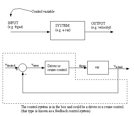
• Control systems use some output state of a system and a desired state to make control decisions.
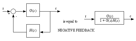
• In general we use negative feedback systems because,
they typically become more stable
they become less sensitive to variation in component values
it makes systems more immune to noise
• Consider the system below, and how it is enhanced by the addition of a control system.
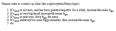
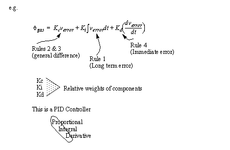
• Some of the things we do naturally (like the rules above) can be done with mathematics
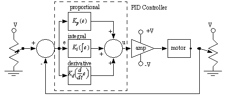
5.1.1 PID Control Systems
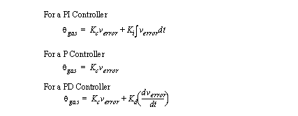
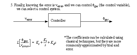
• The basic equation for a PID controller is shown below. This function will try to compensate for error in a controlled system (the difference between desired and actual output values).
• The figure below shows a basic PID controller in block diagram form.
• The PID controller is the most common controller on the market.
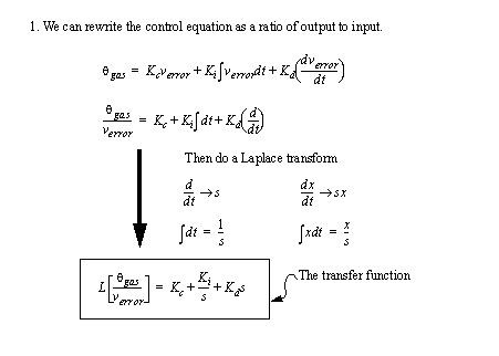
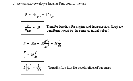
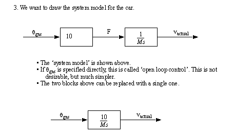
5.1.2 Analysis of PID Controlled Systems With Laplace Transforms
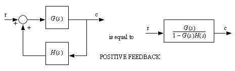
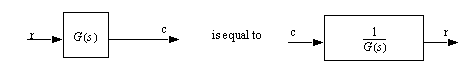
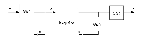
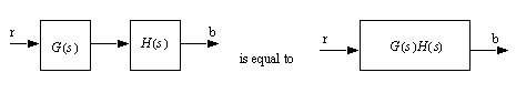
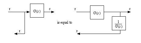
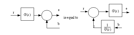
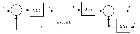
5.1.3 Manipulating Block Diagrams
5.1.3.1 - Commercial PID Tuners
• WARNING: Don’t assume results from these systems are perfect, proper engineering methods must be used to avoid failures in critical systems.
• EXPERTUNE
address
G.E.S.
4734 Soneearhray Dr.
Hubertus, WI 53033
tel: (414) 628-0088
approx. $1500 (U.S.)
will automatically adjust gain and time constant
• LT/TUNE
address
Control Soft Inc.
4122 Wyncote Rd.
Cleveland, OH 44121
tel: (216) 234-5759
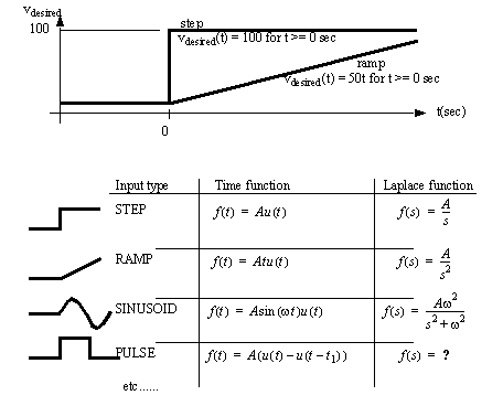
5.1.4 Finding The System Response To An Input
• Even though the transfer function uses the Laplace ‘s’, it is still a ratio of input to output.
• Find an input in terms of the Laplace ‘s’
5.1.5 System Response
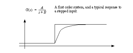
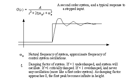
• There are two very common systems assumed: first and second order.
• First order systems are very simple, as is shown below.
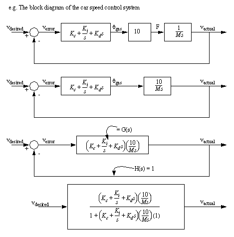
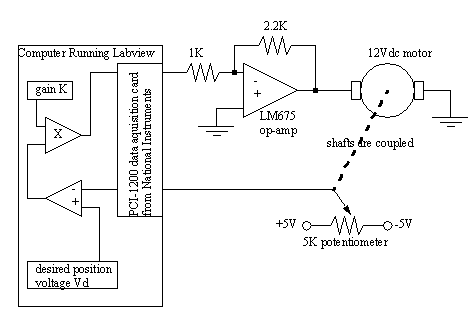
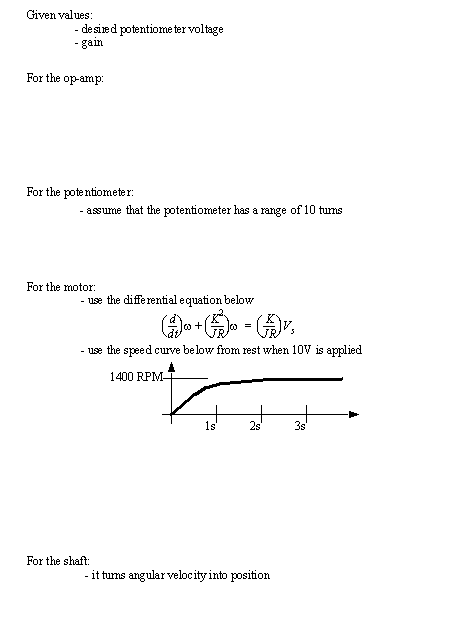
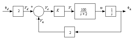
5.1.6 A Motor Control System Example
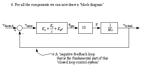
• Consider the example of a DC servo motor controlled by a computer. The purpose of the controller is to position the motor. The system below shows a reasonable control system arrangement. Some elements such as power supplies and commons for voltages are omitted for clarity.
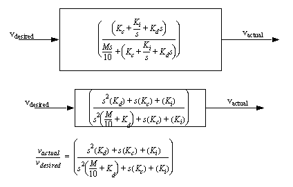
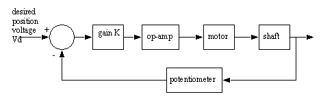
• This system can then be redrawn with a block diagram.
• The block diagram can now be filled out with actual values for the components. Do this below.
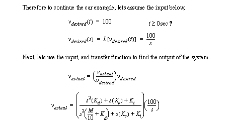
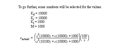
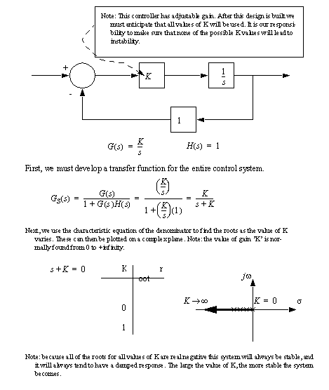
Problem 5.1 Convert the block diagram into a transfer function for the entire system.
Problem 5.2 Pick a value of the gain ’K’ to give a system performance with the damping factor = 1.0.
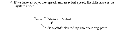
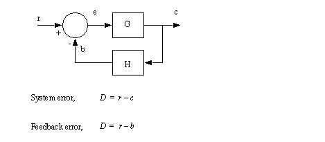
5.1.7 System Error
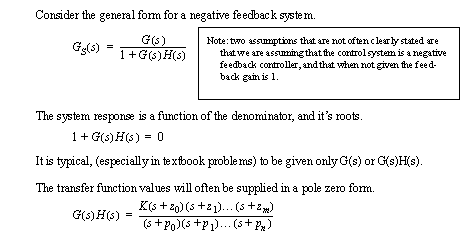
• We typically will be interested in system error and feedback error.
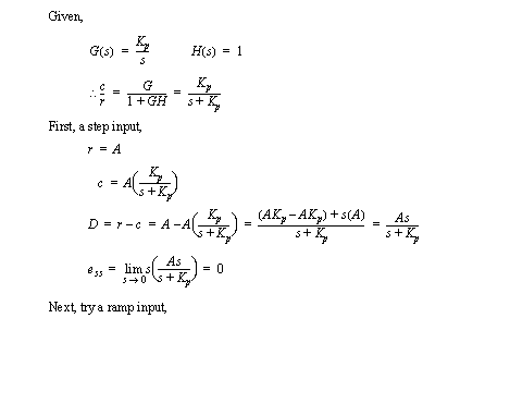
• Consider a simple negative feedback system with various inputs,
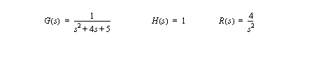
Problem 5.3 Find the steady state system error for the transfer function and ramp below,
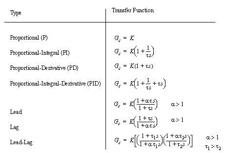
5.1.8 Controller Transfer Functions
• The table below is for typical control system types,
5.2 Root-Locus Plot
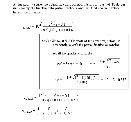
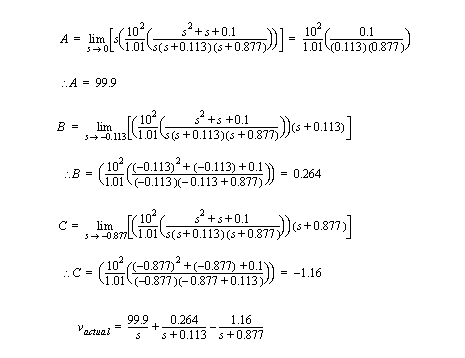
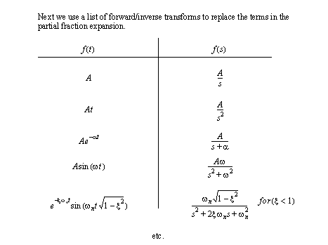
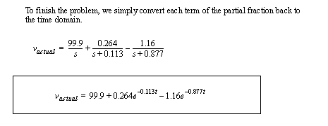
• Consider the basic transform tables. A superficial examination will show that the denominator (bottom terms) are the main factor in determining the final form of the solution. To explore this further, consider that the roots of the denominator directly impact the partial fraction expansion and the following inverse Laplace transfer.
• When designing a controller with variable parameters (typically variable gain), we need to determine if any of the adjustable gains will lead to an unstable system.
• Root locus plots allow us to determine instabilities (poles on the right hand side of the plane), overdamped systems (negative real roots) and oscillations (complex roots).
• Note: this procedure can take some time to do, but the results are very important when designing a control system.
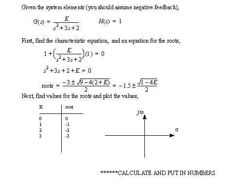
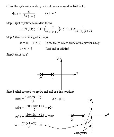
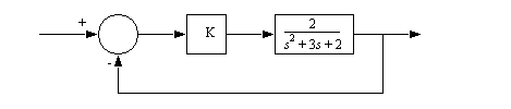
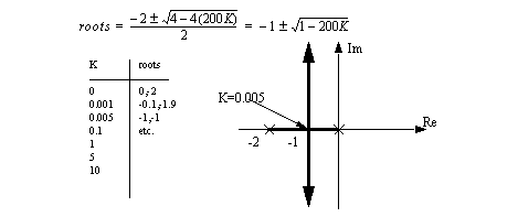
• Consider the example below,
• Consider the previous example, the transfer function for the whole system was found, but then only the denominator was used to determine stability. So in general we do not need to find the transfer function for the whole system.
• Consider the example,
5.2.1 Approximate Plotting Techniques
• The basic procedure for creating root locus plots is,
1. write the characteristic equation. This includes writing the poles and zeros of the equation.
2. count the number of poles and zeros. The difference (n-m) will indicate how many root loci lines end at infinity (used later).
3. plot the root loci that lie on the real axis. Points will be on a root locus line if they have an odd number of poles and zeros to the right. Draw these lines in.
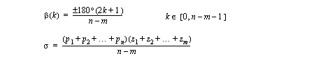
4. determine the asymptotes for the loci that go to infinity using the formula below. Next, determine where the asymptotes intersect the real axis using the second formula. Finally, draw the asymptotes on the graph.
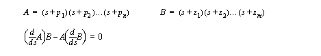
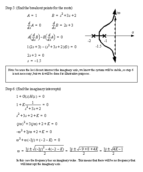
5. the breakaway and breakin points are found next. Breakaway points exist between two poles on the real axis. Breakin points exist between zeros. to calculate these the following polynomial must be solved. The resulting roots are the breakin/breakout points.
6. Find the points where the loci lines intersect the imaginary axis. To do this substitute the fourier frequency for the laplace variable, and solve for the frequencies. Plot the asymptotic curves to pass through the imaginary axis at this point.
• Consider the example in the previous section,
Problem 5.4 Plot the root locus diagram for the function below,
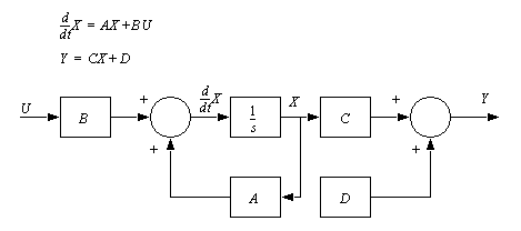
5.2.2 State Variable Control Systems
• State variable matrices were introduced before. These can now be used to form a control system.
5.3 Design of Continuous Controllers
5.4 Problems
Problem 5.5 1. Short answer questions.
a) What is a Setpoint, and what is it used for?
b) What does feedback do in control systems?
c) What is Aliasing and what does it have to do with the Nyquist Criterion?
d) What can A/D and D/A converters be used for in computer control of processes?
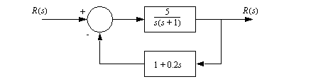
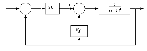
Problem 5.6 Simplify the block diagram below.
Problem 5.7 Given the transfer function below, and the input ‘x(s)’, find the output ‘y(t)’ as a function of time.
Problem 5.8 Find the steady state error when the input is a ramp with the function r(t) = 0.5t. Sketch the system error as a function of time.
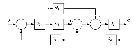
Problem 5.9 Simplify the following block diagram.
Problem 5.10 Given the block diagram below, select a system gain K that will give the overall system a damping ratio of 0.7 (for a step input). What is the resulting undamped natural frequency of the system?
Problem 5.11 What is the transfer function for a second order system that responds to a step input with an overshoot of 20%, with a delay of 0.4 seconds to the first peak?
Problem 5.12 Draw a detailed root locus diagram for the transfer function below. Be careful to specify angles of departure, ranges for breakout/breakin points, and gains and frequency at stability limits.
Problem 5.13 Draw the root locus diagram for the system below. specify all points and values.
Problem 5.14 Draw the root locus diagram for the transfer function below,
Problem 5.15 Draw the root locus diagram for the transfer function below,
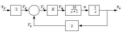
Problem 5.16 The block diagram below is for a motor position control system. The system has a proportional controller with a variable gain K.
a) Simplify the block diagram to a single transfer function.
b) Draw the Root-Locus diagram for the system (as K varies). Use either the approximate or exact techniques.
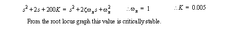
c) Select a K value that will result in an overall damping coefficient of 1. State if the Root-Locus diagram shows that the system is stable for the chosen K.
Answer 5.16 a)
b)
c)
Problem 5.17 Draw a Bode Plot for either one of the two transfer functions below.
Problem 5.18 The block diagram below is for a servo motor position control system. The system uses a proportional controller.
a) Convert the system to a transfer function.
b) draw a sketch of what the actual system might look like. Identify components.
Problem 5.19 Given the system transfer function below.
a) Draw the root locus diagram and state what values of K are acceptable.
b) Select a gain value for K that has either a damping factor of 0.707 or a natural frequency of 3 rad/sec.
c) Given a gain of K=10 find the steady state response to an input step of 1 rad.
d) Given a gain of K=10 find the response of the system as