3. Discrete Systems
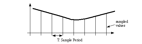
• When dealing with computers we will sample data values from the real world. These sampled values can then be used to estimate how a system will behave.
• The term ‘discrete’ refers to the use of single sampled values, instead of a continuous functions. You will see that the difference is between weighted sums and integrals.
3.1 Modeling With Equations
• We can write a differential equation, and then manipulate it to put in terms of time steps of length ‘T’
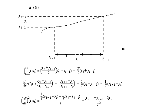
• In review consider how we can approximate derivatives using two/three points on a line.
Problem 3.1 If we read the flow rate of oil in a pipeline once every hour for three hours. The readings in order are 1003, 1007, 1010. What is the integral and first and second derivatives for the values?
3.1.1 Getting a Discrete Equation
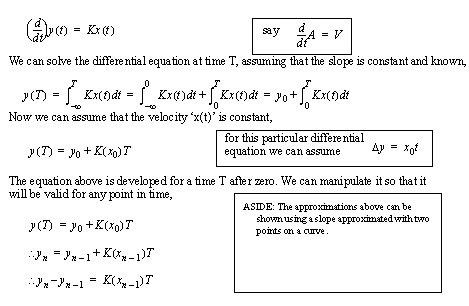
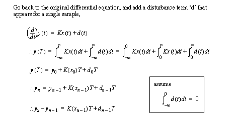
• First, consider the example of a simple differential equation,
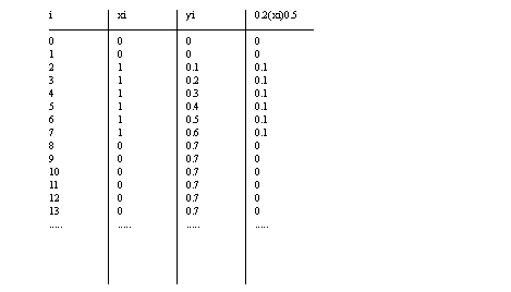
• We can continue the example and use this equation to simulate the system. Here the ‘x’ values are given, and the first ‘y’ value is assumed to be 0. Assume T=0.5 and K=0.2.
Problem 3.2 Find the discrete equation for the differential equation below. Then find values over time.
• We can expand this model by also including a ‘disturbance’. This can be used to model random noise, or changes in system loading, found in all systems.
3.1.2 First Order System Example
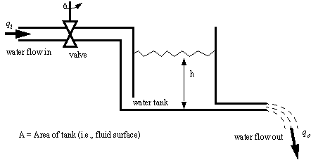
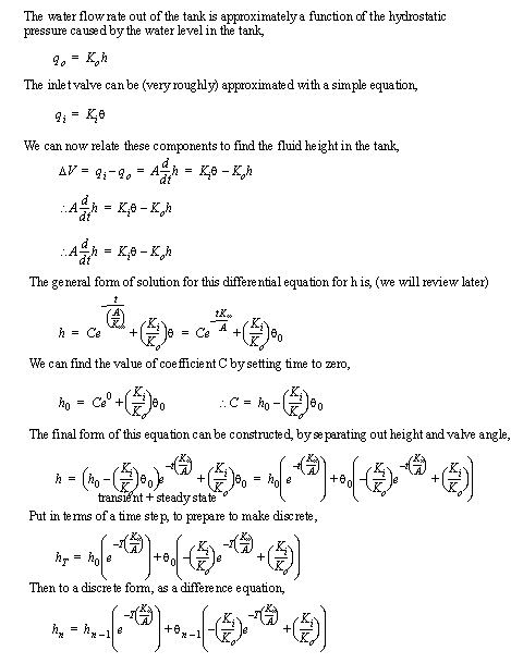
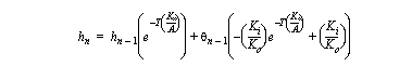
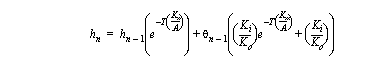
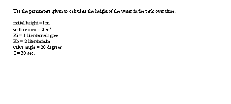
• The water tank below has a small outlet, and left alone the fluid level in the tank will drop until empty. There is a valve controlled flow of fluids into the tank to raise the height of the fluid.
• As long as the fluid levels in the tank are normal, the inlet and outlet flow rates are independent, We can model them both with simple differential equations,
• This difference equation can then be used to predict fluid height. If we change the valve position, this will also be reflected in the calculated values.
egr450.0.mcd
Problem 3.3 Now try varying the input valve angle using all of the conditions outlined before, find out what happens when the valve angle is changed to 10 degrees after 10 seconds.
3.1.3 Second Order System Example
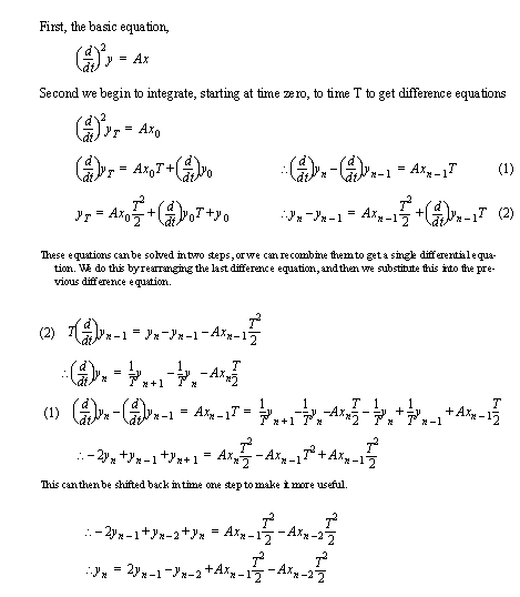
• Consider the second order example below,
Problem 3.4 Calculate the position of a 5 Kg mass if a force of 2N is applied for 5 seconds and then removed. Try the calculations using a 1 second and a 2 second period.
3.1.4 Example of Dead (Delay) Time
• In a real system there is a distance between an actuator, and a sensor. This physical distance results to a lag between when we actuate something, and when the sensor sees a result.
• Assume we have a simple process where after a change in x there is a delay of ‘m’ time steps before the proportional change occurs in y. We can write the equation as,
Problem 3.5 Calculate the position of a 5 Kg mass if a force of 2N is applied for 5 seconds and then removed. There is a one second delay between the time that the force is applied, and when the effects are apparent on the mass.
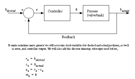
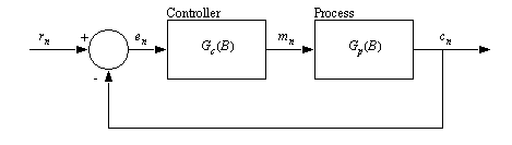
3.2 Discrete Controllers
• The system models we developed before allow us to predict how a system will behave. A separate, and important topic is computer control.
• With no controller we would set an input, and hope for an output. For example, push the gas pedal and hope for the right speed.
• A controller looks at the desired system condition, and the actual system condition, and then adjusts the input to bring the desired and actual closer. For example cruise control.
• The diagram below is a representation of a simple control system add to in the previous tank example,
• We have already dealt with deriving an equation for the process. In this case it was the valve tank combination discussed before. By itself the tank is an open loop system, we set the valve angle and hope for a liquid level.
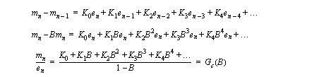
•Next, we need to find an equation for the controller. This equation can be highly dependent upon the control method to be used. If we are to use a computer it is best to have a simple equation, as shown below, (NOTE: the form of the equation, and the values of the coefficients change the nature of the control problem).
• The controllers (equations) that follow will be put in the above form. These controllers can also be used individually, or combined to get more complex properties.
• Keep in mind that the typical objective of a control system is to minimize the error between the input and output. Another common goal is to do this as quickly, or efficiently as possible. One constraint we must observe is that the system should not become unstable.
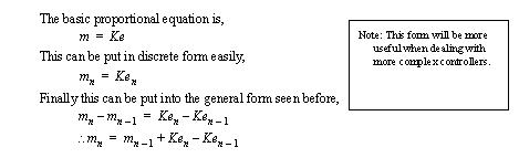
3.2.1 A Proportional Controller
• One of the simplest controllers is the proportional control,
• The magnitude of K will determine how fast the system responds. If the value is too large the system will oscillate and/or become unstable (i.e. flood or go empty). If too small the system error will be very large. (ie, the tank will never reach the right height.)
• This type of controller will always have a small error between the actual and desired values.
Problem 3.6 For the water tank (from before) add a controller, and try varying ‘K’ values.
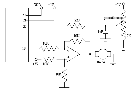
• We could implement this controller using the Basic stamp chip. (Note: not a full implementation)
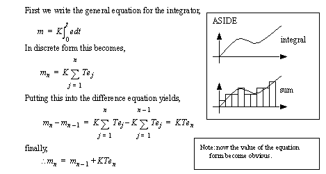
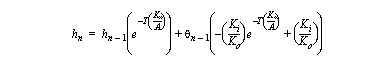
3.2.2 Integral Control
• Integral controllers tend to respond slowly at first, but over a long period of time they tend to eliminate errors.
• The integral controller is based on a simple integration.
• If the constant K is small, the longer term error will slowly drop off. If K is large the long term error will be reduced quickly. Too large a K value will result in a signal that grows out of control.
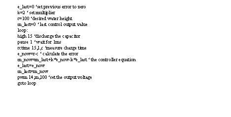
Problem 3.7 Try controlling the water tank with the I controller,
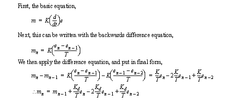
3.2.3 Differential Control
• When there is a sudden change in the system the differential controller will be able to compensate. But in terms of long term effects the controller will allow huge steady state errors.
• The control equation can be derived as,
• This larger the value of K the faster this controller will compensate for a change in the system.
Problem 3.8 Try controlling the water tank level with the D controller,
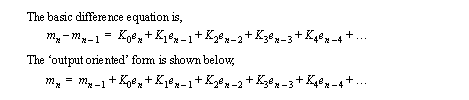
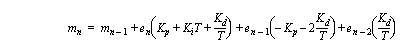
3.2.4 Proportional, Integral, Derivative (PID) Control
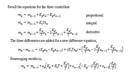
• The functions of the individual proportional, integral and derivative controllers are complementary. When combined we get a system that responds quickly to change (derivative), generally track required positions (proportional), and will eventually reduce errors (integral).
• To get this we combine the expressions from the three individual controllers. Subscripts will be added to distinguish the ‘K’ gain values for each controller.
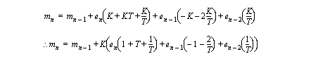
• Quite often the three constants are made the same, giving us the simpler equation below.
• This controller now allows us to vary the three different gains, and as a result we will change the performance of the system.
Problem 3.9 Given the water tank from before (with the given variables), try a variety of different values for the PID gains to see how the system responds.
egr450.1.mcd
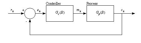
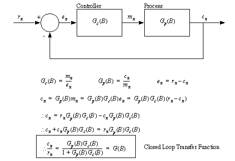
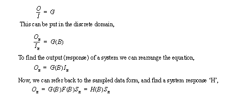
3.3 Block Diagrams and Transfer Functions
• Block diagrams are the primary tool for showing process and control system models.
• In a block diagram each block has one input and one output.
• A transfer function provides functions that are a ratio of block output to block input.
• Consider the block diagram seen before, but with transfer functions (ratio of output to input) shown for the controller and process.
• Both of the transfer functions are ratios of inputs to outputs,
• These transfer functions (ratios) are rarely a simple multiplication, and so we need to use an alternate representation called a ‘transform’.
• In this case we will use a backshift transform, hence the ‘B’ in the representation.
Problem 3.10 a) Develop equations for the block diagram below,
b) Recall and apply the techniques for block diagram manipulation.
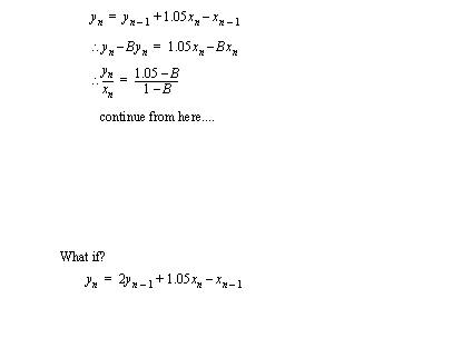
3.3.1 The Backward-Shift ‘B’ Operator
• An operator is a special part of an equation: one example is the (d/dt) of calculus.
• The basic definition of the backshift operator ‘B’ is,
• If we apply this operator to an equation seen before,
• This form then allow some very useful techniques that we will see later.
Problem 3.11 Apply the ‘B’ transform to the PID expression found before,
Problem 3.12 Apply the ‘B’ transform to the valve and water tank found before,
3.3.2 Reducing Block Diagrams
• A useful method for this form is the ratio of the actual output to the desired output, (c/r)
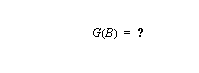
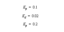
• If we are planning on applying the PID controller to the water tank example from before we get the following block diagram, (Note: the block diagram is overkill in this application)
Problem 3.13 Find the closed loop transfer function for this process and controller,
Problem 3.14 For the problem below, use the PID values, with the valve/tank parameters used previously to find the system response to a step input to 20 at time zero, and 10 at time 10. (hint: convert the closed loop equation back to a difference equation)
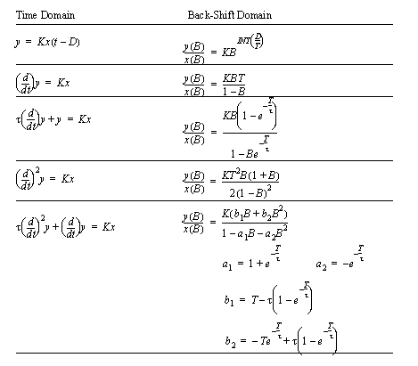
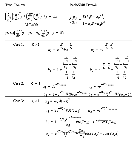
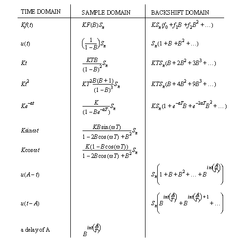
3.3.3 Back-Shift Transform Table
• The general application of the table is,
1. Develop the differential equation.
2. Look for the equation in the table. Sometimes the equation will have to be rearranged to match the form in the table. If it is not in the table, derive the transfer function the long way.
3. Select the appropriate transfer from the right column, and substitute in values and variables.
• A few of the transforms are given below,
Problem 3.15 Find the transfer function for the system below,
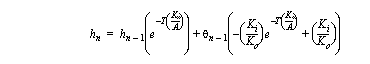
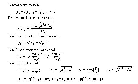
3.3.3.1 - A Summary of Differential Equation Solutions
• A quick look at how differential equations relate to difference equations will be useful.
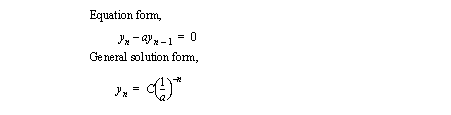
• First order homogeneous difference equation,
• second order homogeneous difference equation,
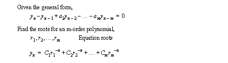
• Higher order homogeneous difference equations,
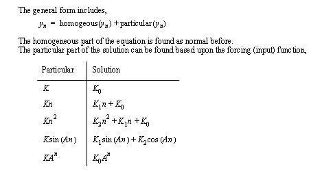
• non-homogeneous equations
Problem 3.16 Solve the following differential equation
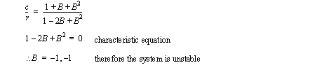
3.3.4 Stability
• Basically a system will become unstable if a transfer function starts to grow. We can predict this by looking at the characteristic equations.
• The characteristic equation is the denominator of the transfer function.
• If any of the roots of the equation are less than one, then the system can become unstable, and most likely will.
Determine if the function below is stable, if y is the output,
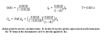
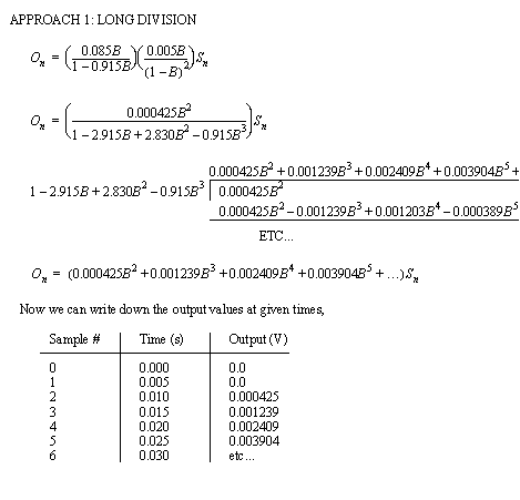
3.4 Sampling Functions
• In the last section we looked at a technique for writing equations for discrete variable values. This section will start to relate this to the design of controllers and control algorithms.
• Although hinted at earlier, we can now formally define a value ‘sampled’ into the computer. These values are taken in such a short period of time that they are effectively instantaneous. But this means that the value does not include changes between samples, and is particularly prone to noise.
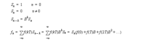
• The unit sample has a magnitude of 1 (and can be multiplied by an input magnitude). The subscript can be used to shift it in time. We can relate in the backshift operator, and finally use it to represent input (generating) functions,
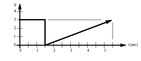
Problem 3.17 Develop the expression for the following function assuming a sampling time of 1 s, and then assuming 0.5 s.
• Table of sampling functions,
Problem 3.18 Try the previous example using the lookup table,
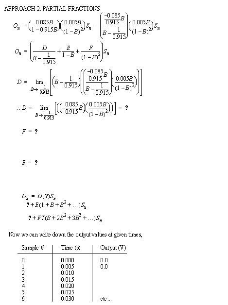
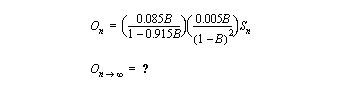
3.5 System Response
• Consider that the general form for a transfer function is,
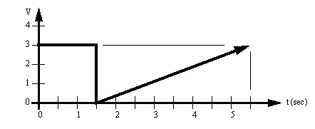
• We can try an example to estimate how a system would respond,
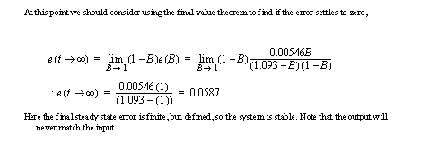
• Sometimes we don’t want to see the initial changes (transients), but we are more interested in the long term final value (steady state). We can use the final value theorem to find this,
Problem 3.19 Consider the previous function,
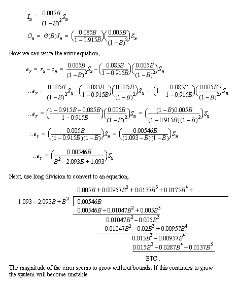
3.6 Steady State Error
• When we examine a controller, we may look at the value of the error function into the controller.
• If the value of the error function does not become zero at infinity, the system is unstable.
• We can calculate the error value using the function,
• If we consider the example from before,
3.7 Problems
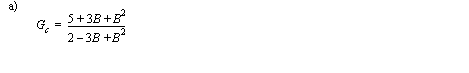
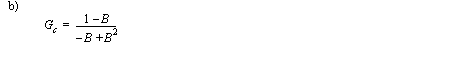
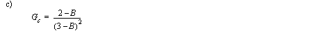
Problem 3.20 Develop a discrete equation for the following transfer functions. Determine stability and realizability.
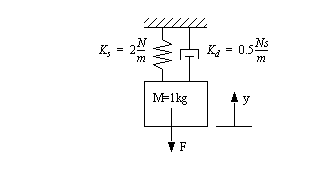
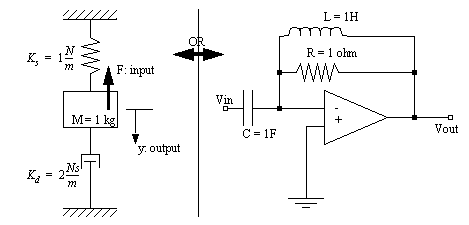
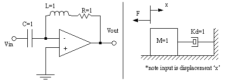
Problem 3.21 Develop a differential equation for both the mechanical and the electrical system below. Find the transfer function for the module using the backshift operator ‘B’ for a time step of T = 1 sec.
Problem 3.22 a) Given the following transfer function, and the input function, find the resulting output for the first 5 time steps, if T=0.5 seconds.
b) What will the steady state output be for the system in part a)?
Problem 3.23 Develop a process model for one of the systems below. Assume the system starts at rest.
a) Write the differential equations for one of the systems above.
b) Convert the equation to a transfer function using the backshift operator (use T=1sec).
c) Assume there is a step input of magnitude 1. Find the output function for the system in terms of the backshift operator. Do not convert the output function to numerical values in time.
d) Determine the steady state value for the system. Is the value consistent with what you would expect from the system? Explain.
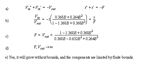
Answer 3.23
Problem 3.24 Given the following output function,
a) Find the steady state response as a function of time using the tables (assume T=0.2sec).
b) Find the first three values of the output in time using long division. Check that these values agree with the solution found in part a).