13. System Responses
• We can categorize certain systems into well known divisions. In many cases this will permit some back of the envelope calculations.
• When we consider responses we look at the type of input applied. These typically include,
step
ramp
parabolic
sinusoidal
• The most common analysis involves applying a step function to the system. The type of response tells us a great deal about the nature of the system.
first order: a simpler system that tends to be made of passive components and will come to rest
second order: a system that has natural frequencies
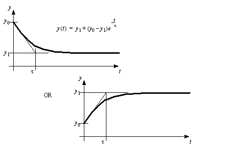
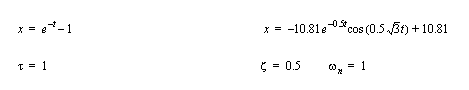
13.1 First Order Step Responses
• A step input implies that there is a sudden change in an input. These are very commonly used to check the behavior of a control system. And most systems operate with stepped changes in values.
• These systems follow the general form of exponential decay.
• Note: the curve above could also go up (just change the values).
• These systems are common for simple systems that do not have energy sources. These systems don’t vibrate by themselves, unless shaken periodically.
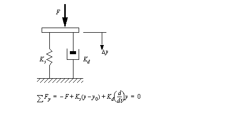
• Consider a first order equation for the position of a spring damper system. Complete the solution.
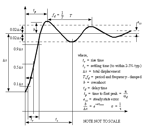
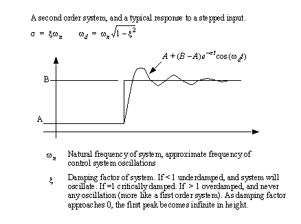
13.2 Second Order Step Responses
• Second order systems tend to have a first order decay, but they also have a sinusoidal component.
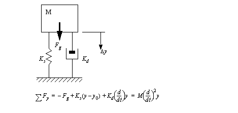
• Consider the example,
• These systems have a well know time function, as is pictured below. This particular response is for a step input function.
• These systems are commonly described using the natural frequency and the damping coefficient.
• Consider the example,
13.3 Other Responses
• When we have a system that doesn’t have the form of a first or second order system, or our input is other than a step function, we need to calculate the response.
• The response of the systems is calculated by solving the differential equations.
• To solve the equations we could use the Runge-Kutta technique, or solve the differential equations.
13.3.1 Solving Differential Equations
• Please refer to the relevant section in the math handbook.
13.3.2 Complex Numbers
• Please refer to the relevant section in the math handbook.
13.4 Response Analysis
• After doing an analysis of the response, it is important to examine the results to determine their importance.
• Some general notes,
1. If a step input causes the system to go to infinity, it will be inherently unstable.
2. A ramp input might cause the system to go to infinity, if this is the case the system might not respond well to constant change.
3. If the response to a sinusoidal input grows with each cycle, the system is probably resonating, and will become unstable.
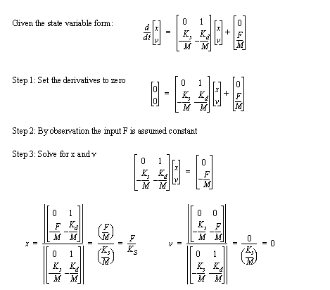
13.5 Steady State and Equilibrium
• The steady state of a system is the value it will take after all of the initial (transient) effects have occurred.
• This can be done by,
1. Setting all derivatives to zero in the state variable form
2. Ensure all inputs are constants
3. Solve the equations
• Consider the steady state solution of the problem below,
• NOTE: Use this technique with a great deal of caution. Steady state does not imply sitting still, just that initial effects (transients) have settled out. This technique does not recognize systems that have settled into states of periodic motion.
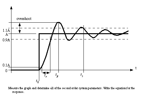
13.6 Problems
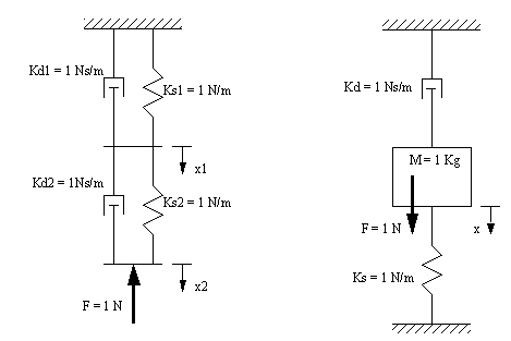
Problem 13.1 a) Write the differential equations for the system below. Solve the equations for ‘x’ assuming that the system is at rest and undeflected before t=0. Also assume that gravity is present.
b) State whether the system is first or second order. If the system if first order find the time constant. If it is second order find the natural frequency and damping ratio.
Answer 13.1
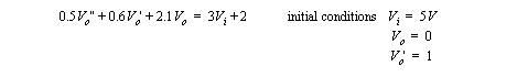
Problem 13.2 a) Given the following differential equation and initial conditions, draw a sketch of the first 5 seconds. The input is a step function that turns on at t=0.
b) Solve the same problem as in part a) using explicit integration to get an equation that is a function of time.