BCAPP - A High Level Process Planner Using Boolean Algebra
by H. Jack
ABSTRACT
Years of process planning research has lead to a number of successful approaches, which include the existing Computer Aided Process Planning (CAPP) systems that can be described as experts for specific manufacturing processes. This has created a need for high-level process planners that simultaneously considers multiple manufacturing technologies.
A process planner called BCAPP (Boolean CAPP) is described. It uses a Boolean algebra based design representation to develop a high level process plan. The system then relies on other process planners to do detailed (low level) planning and estimate time standards for each operation. Some additional features of interest in this system are; generation of alternative operations, the use of cost estimates, new technologies are easily incorporated, uses hierarchical planning techniques are used to reduce the search space, and it is capable of recovering from plan failures.
1.0 INTRODUCTION
Computer Aided Design (CAD) systems take direction from a user that direct the construction and analysis of a geometrical model. At present, the geometrical model of the product is preserved, while the steps of creation are discarded. When the steps of creation are preserved they provide clues about the manufacture of a product. A product definition was developed that maintains the definition steps, as opposed to explicit geometry using Boolean equations and sets. The Boolean equations allow the basic operations found in solid modellers, such as subtraction, intersection, union, and assembly. The sets carry the fundamental information about the geometry, such as shape, dimensions, position and orientation. This approach allows attributes to be assigned that are difficult to associate with traditional CAD models.
The Boolean equations of the design representation can be converted to a set of production steps to form the basis of a process plan. (The process plan is not unique for a design equation. Each design equation and its sets are not unique to a specific design [4]). The fact that these plans are not unique is often seen as a problem when using these methods. However, when process planning, the process plan will vary as conditions of production equipment and other essential resources change. This dictates that the process planner be able to consider alternate plans, as is done in any successful planning approach. The non-uniqueness of the design representation is used to allow the Artificial Intelligence (AI) planning routines to generate alternative operations. The planner will find alternatives from a single equation, and if unsatisfied it will request equivalent Boolean equations that will be generated using the rules of Boolean algebra. A similar approach was used by Lee [4].
The planning algorithm uses a number of strategies to search for locally optimal solutions. In general the operation of the planner is of the form i) equation pattern recognition, ii) condition evaluation of implicated sets, and iii) application of best match rules.
2.0 THE NATURE OF DESIGNS
A design embodies structures, especially those related to function. These physical constructs have design features that range from basic geometrical primitives (e.g. box shape), to complex features (e.g. counterbored holes), to highly abstract properties (e.g. color). The full range of these design features are simultaneously used in most designs. For example, a countersunk screw is a cylindrical shaft (primitive) with a threaded shaft (feature) and a cone (primitive) with a slot (primitive) cut out. The screw is brass colored (abstract) for aesthetic reasons.
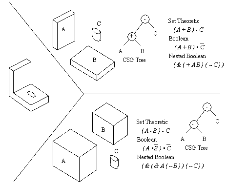
Figure 1.1 Alternate Data Structures for Solid Models
The extensive list of existing solid modelling techniques [5][2] address the designs on a primitive level very well. Complex features can also be modelled well, but these can be difficult to recognize once the object is modelled. Abstract features can be associated with the models if they can be linked to faces, vertices, edges, etc. A concurrent representation of modelled geometry and abstract design are needed for a good design representation. The design method chosen is a generalization of the CSG (Constructive Solid Geometry) model. And, being CSG-like, it can be used to produce a boundary representation (B-Rep) model [2]. The basic elements of the representation are sets to hold information and Boolean equations to apply them. The set membership is not specified at this time, and can be eventually matched to the rules selected. This statement can be emphasized by the use of the method to represent both mechanical parts, and digital circuits [3].
The use of Boolean equations instead of CSG trees allows access to the well understood laws of Boolean algebra, and allows simplification of the complex operators in CSG (e.g. subtraction). Further extensions have been incorporated to allow more practical modelling. First, a nested equation form was used to clarify operator scope for the user, and to formalize the data structures. This form is shown in Figure 1 below, and can be seen to be equivalent to an expression that is not nested (i.e. it only involves the addition of parenthesis). Second, additional set properties can be appended to sets or terms in the equation. This allows reuse of sets when designing, or the addition of abstract properties to groups of geometrical features. This handling of groups is not easily done in other representation methods and causes great problems when modelling tolerances and other abstract properties.
3.0 RECOGNITION OF MANUFACTURING FEATURES AND PLANNING WITH THEM
3.1 A SIMPLE EXAMPLE
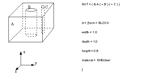
Assume a design is given (in Figure 2) for a square nut, with a threaded, and an offset hole.
Figure 1.2 A Simple Part Design with Nested Boolean Representation
In this example we see the nut as a block (A) with a tapped hole (B) removed and hole (C) removed. The block A and hole C are defined as primitives, and the hole B is defined as a feature.
We can see how B is different from A and C: During planning we would first look for certain algebraic forms in the equation. In this case the general form ‘( & X0 X1 X2 ....... ( ~ Y1 ) ....’ suggests Y1 is removed from ‘( & X0 X1 X2 .....’. Here we see that B is to be removed from A. In the second phase the sets A and B must be examined. If B was a simple hole with dimensions only it would probably be drilled. This would also rely on the geometric validity of the operation (i.e. the centre line of the drilled hole must be normal to the surface). In this case B contains the property ‘tapped = 5/8-11-UNC’ which would fire a rule for cutting threads. The results of the rule application would be the addition of a tapping operation to the process plan, and the replacement of set B with a new set.

The planning would then continue, and this time B1 will be recognized as a simple drilled hole. (We shall address the recognition process in the next section.) The drilling rule would be applied, and a drilling operation added to the process plan. The equation term containing B1 would now be deleted and the design equation would become,
The planning would continue with the recognition of removed hole C. This time when C and A are examined the basic drilling rule would not fire because of the tolerance, but a reaming rule would. This rule would add a reaming operation to the process plan, and replace set C with an updated set.
Next, set C1 does fire the hole drilling rule, a hole is drilled, and the equation reduced.
Finally, the equation matches a simple primitive template. This fires a stock cutting rule and a process step for stock cutting is added and the NUT equation is reduced to NULL. (If the nut tolerances existed a milling operation might have been added.)
The final process plan for the part is,
Notice the order of the plan is reversed from the backwards sequence of planning.
4.0 THE DETAILED METHOD
The previous section described the method in general, ignoring many of the underlying technical issues. The following sections are targeted at explaining how some of the complicated tasks have been accomplished.
4.1 TEMPLATE MATCHING
In the previous example, sections of the equation were “recognized”, and these recognized terms in the expression were subsequently examined with rules. A simple pattern matching scheme was used to extract these terms. Simplistic templates are used to identify useful forms in the equations. Some template elements and a few example templates are given below.
( X Start of a term, where ‘X’ is ‘?’ for any operator, or ‘+, &, :, ~’
for a specific operator.
) End of a term.
VAR:name:i Refers to a variable list of all sets within a term (not including sets).
VAR:name:x As above, but where the variable is ‘x’ integer positions from the start.
(> This refers to the start of the total expression only.
...( Allows a list of variables to be ignored before the start of a term.
...) Allows a list of variables to be ignored before the end of the term.
):LABEL:X Allow a variable ‘X’ name to be bound to a term.
):VAR:X Assigns all of the properties of a term to be given a variable name.
VAR:name:i:prop Assigns the properties of a variable as well as the normal symbol assignment.
Figure 1.3 Equation Templates and Valid Match Examples
The templates are only conditional, and are not very sophisticated, but are sufficient to recognize most equation patterns (future work is required). After templates are matched, they suggest rules for comparison. This also explains the use of variables in the template. For example, in Figure 3 the variable A0 is A, A1 is B, and B0 is C. When rules are selected they refer to A0, A1 and B0, and the sets A, B, and C are indirectly examined.
The algorithm for finding template matches will examine all possible combinations in the equation. When the algorithm is complete all possible matches will have been found. These templates allow pruning of the search space, and high level extraction of possible processes. The templates also allow a single rule to be fired for alternate templates thus reducing redundancy.
4.2 RULES
While the templates suggest possible processes, they are not sufficient. To ensure the equation and sets satisfy the conditions, simple if-then production rules are used. The rules examine the properties in the sets, and if all rule conditions hold, the actions are performed. The actions typically include equation modification, creation of new sets, and creation of process plan steps. As the actions transform the design, the process plan is expanded, and the design is reduced. A set of design rules are seen later on, some of the operator actions are described below.
EQUATION_INSERT_SYMBOL - This will insert a symbol (a set name) at a specified position in an active expression.
EQUATION_DELETE_SYMBOL - This function will delete a set name that is at a specified location.
EQUATION_DELETE_TERM - A term at a specified location will be deleted.
EQUATION_DELETE_VARIABLE_TERM - This will delete a term that has been given a label using the ‘LABEL’ operator in the template matching string.
EQUATION_INSERT_TERM - A given term will be inserted at the given position in the current expression.
COPY_SET- This simply copies one set to a new set.
ADD_SET- This function creates a new set.
ADD_PROPERTY - This function will add a property to a set.
PROPERTY_FUNCTION_VARIABLE - Performs a mathematical operation based on set members.
PROPERTY_FUNCTION_NUMBER - Performs a mathematical operation based on a set member, and a number.
DELETE_PROPERTY - A specified property will be deleted.
PLAN_PUSH_TEXT - Adds a line of test to the process plan.
PLAN_PUSH_FORMAT - Adds a line of text to the process plan, but using a formatted output. This allows the use of variables in plan output.
DECLARE_COST - A numerical cost is declared, so that the system may perform some process selection based upon the cost of operations.
PROPERTY_FUNCTION_VARIABLE - Perform a math function based upon two variable names.
PROPERTY_FUNCTION_NUMBER - Perform a math function on a variable with a number.
FIND - This function allows complicated operations to be performed, such as the lookup of the cost of a material, or a geometric property. Many complex functions can be added through this device.
The example rule file shown below has four main components; equation templates, rule conditions (antecedents), and rule results (consequents). The ‘equation_form’ shown has the equation template, and rules that it may fire when matches occur. The ‘rule’ definitions have a condition equation and results to fire when the equation is valid. The equation is a simple logical expression that refers to the truth of the ‘condition’ definitions. The conditions allow simple calculations, database references, and compares. Finally the ‘result’ definitions describe functions that may be performed. In general the results alter the equations, add new sets and properties, specify estimated costs of operations, and add operations to the process plan.
equation_form EQN_1 {
EQUATION: ( & ...( ~ VAR:V:0 ):LABEL:REF
RULE: drill_hole
RULE: chamfer_drill
}
equation_form EQN_9 {
EQUATION: (> : VAR:V:0 VAR:V:1 ...)
RULE: assemble_parts
}
rule assemble_parts {
EQUATION: ( & PART_0_EXISTS PART_1_EXISTS )
RESULT: ASSEMBLE_PARTS
}
rule drill_hole {
EQUATION: ( & CYLINDER_SHAPE DRILL_SIZE )
RESULT: DRILL_HOLE
}
rule chamfer_drill {
EQUATION: ( & CONE_SHAPE DRILL_SIZE )
RESULT: DRILL_CHAMFER
}
condition PART_0_EXISTS {
COMPARE ( V0.form $ )
}
condition PART_1_EXISTS {
COMPARE ( V1.form $ )
}
condition CYLINDER_SHAPE {
COMPARE ( V0.form == CYLINDER )
}
condition CONE_SHAPE {
COMPARE ( V0.form == CONE )
}
condition DRILL_SIZE {
MATH ( V0.ratio = V0.height / V0.radius )
ASSIGN ( V0.minimum = 0.5 )
COMPARE ( V0.ratio > V0.minimum )
COMPARE ( V0.ratio < 20 )
COMPARE ( V0.radius > 0.05 )
COMPARE ( V0.radius < 2.5 )
COMPARE ( V0.height > 0.1 )
COMPARE ( V0.height < 15.0 )
}
result DRILL_HOLE {
EQUATION_DELETE_VARIABLE_TERM ( REF )
ADD_SET ( DRILL_HOLE )
ADD_PROPERTY ( DRILL_HOLE a1 = 0.5 )
ADD_PROPERTY ( DRILL_HOLE a2 = 1.0 )
ADD_PROPERTY ( DRILL_HOLE height = 0.0 )
PROPERTY_FUNCTION_VARIABLE ( DRILL_HOLE height + V0 height )
PROPERTY_FUNCTION_NUMBER ( DRILL_HOLE height / 20.0 )
PLAN_PUSH_TEXT ( ‘ DESCRIPTION ( drill hole ) ‘ )
PLAN_PUSH_TEXT ( ‘ CUTTING ( FEATURE single diameter hole ) ‘ )
PLAN_PUSH_TEXT ( ‘ CUTTING ( MACHINE qa1000 ) ‘ )
PLAN_PUSH_TEXT ( ‘ CUTTING ( MATERIAL t-7075 ) ‘ )
PLAN_PUSH_FORMAT ( ‘ CUTTING ( PARAMETERS ‘ DRILL_HOLE.height
DRILL_HOLE.a1 DRILL_HOLE.a2 ‘ ) ‘ )
// A costing section is added here for a trial run
ADD_PROPERTY ( DRILL_HOLE cost = 0.0 )
PROPERTY_FUNCTION_VARIABLE ( DRILL_HOLE cost + V0 height )
PROPERTY_FUNCTION_VARIABLE ( DRILL_HOLE cost * V0 radius )
PROPERTY_FUNCTION_NUMBER ( DRILL_HOLE cost * 1250.25 )
PROPERTY_FUNCTION_NUMBER ( DRILL_HOLE cost + 0.25 )
DECLARE_COST ( DRILL_HOLE cost )
}
result DRILL_CHAMFER {
EQUATION_DELETE_VARIABLE_TERM ( REF )
ADD_SET ( CHAMFER_HOLE )
ADD_PROPERTY ( CHAMFER_HOLE a1 = 0.5 )
ADD_PROPERTY ( CHAMFER_HOLE a2 = 1.0 )
ADD_PROPERTY ( CHAMFER_HOLE height = 0.0 )
PROPERTY_FUNCTION_VARIABLE ( CHAMFER_HOLE height + V0 height )
PROPERTY_FUNCTION_NUMBER ( CHAMFER_HOLE height / 20.0 )
PLAN_PUSH_TEXT ( ‘ DESCRIPTION ( drill chamfer ) ‘ )
PLAN_PUSH_TEXT ( ‘ CUTTING ( FEATURE Front Countersunk Hole ) ‘ )
PLAN_PUSH_TEXT ( ‘ CUTTING ( MACHINE qa1000 ) ‘ )
PLAN_PUSH_TEXT ( ‘ CUTTING ( MATERIAL t-7075 ) ‘ )
PLAN_PUSH_FORMAT ( ‘ CUTTING ( PARAMETERS ‘ CHAMFER_HOLE.height
CHAMFER_HOLE.a1 CHAMFER_HOLE.a2 ‘ ) ‘ )
}
result ASSEMBLE_PARTS {
EQUATION_DELETE_TERM ( :1 )
PLAN_PUSH_TEXT ( ‘ DESCRIPTION ( add part to fixtured part ) ‘ )
}
Figure 1.4 Sample of a Rule File
4.3 THE PLANNER
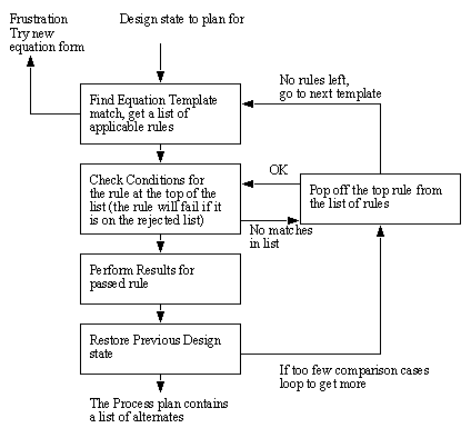
The large number of possible solutions makes the direct application of rules infeasible, leading to the conclusion that a pruned search space is required. In addition, the temporal nature of the problem suggests that a planner is best suited to the problem. The planner uses a hierarchical two-step application of template pattern matching, and then rule checking.
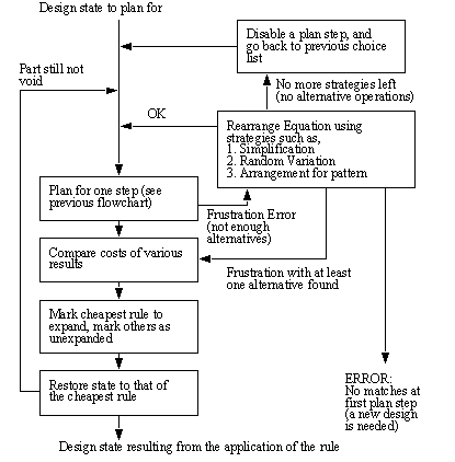
After application of the rules, many possible processes can be identified after the matching phase, and estimated costs can be used to choose between them. Also, certain techniques have been used to approach the non-linear and time variant nature of the plans. One approach involves backtracking. As the plan is developed, a tree of plan steps is completed. If a blind alley is encountered, or a plan step becomes invalid because conditions in the factory change, the planner will go back and try alternate operations. All of the alternate steps are contained in the process plan, so that a scheduler can make use of alternate plans when required. A second technique that deals with plan sequence non-linearity is the manipulation of the Boolean equations. When the planner is unable to find enough valid operations for a specific production state, it will simplify, or randomly change the equation. Eventually other manipulation strategies will be enabled for the Boolean equations. Essentially by reseeding the planner, we can now get around solutions locked in a certain goal, much as a random walk technique would in traditional optimization problems. Two flow charts are given in Figures 5 & 6 that outline the basic strategies of the planners.

Figure 1.5 High Level Planning
Figure 1.6 Low Level Planner
5.0 RESULTS
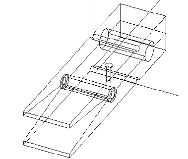
The results presented here have been chosen to illustrate the diverse planning capabilities of BCAPP. The first product described is an advertising paperclip in the form of an oversized clothespin. In this design there are some interesting features.
• There are two identical halves of the clip, except that one side has a logo added, and a mounting hole drilled.
• The process used in production are machining, metal forming, assembly, and embossing.
• The geometry is not entirely defined as illustrated by the replacement of the spring to join the halves with a tube. The spring was defined as a feature, not as a geometry.
Figure 1.7 A Test Part - A Large Plastic Clothes Pin
The process plan for the large paperclip is given below, and was generated in entirety by BCAPP.
-------- Work Order Sheets ------------
Product: Big_Clothes_Pin
OPERATION SUMMARY_SHEET: Clip_half_PART - Quantity 2.000000
OP# Operation Description
------------------------------------------
0 cut a block from stock
width = 1.4
depth = 5.9
height = 0.55
10 drill hole : D
20 drill hole : C
30 drill hole : B
40 mill out block shape : E
Figure 1.8 Process Plan for the Big Clothes Pin
Some items of note about the plan are listed.
• The plan uses drilling operations for holes on the clip half, but drilling would fail because the bit would deflect. This will be overcome when solid modelling capabilities are added (currently being investigated).
• The planner recognized the need for 2 clip halves, instead of producing 2 separate plans.
• The plan steps address high level process selection. Other process planners can provide detailed plans for each specific process.
OPERATION SUMMARY_SHEET: 0:Logo_Side_PART - Quantity 1.000000
OP# Operation Description
------------------------------------------
1000 get WIP from inventory
name = Clip_half
1010 drill chamfer
1020 drill hole : COMBINED_SET_10
OPERATION SUMMARY_SHEET: Logo_Side_PART - Quantity 1.000000
OP# Operation Description
------------------------------------------
2000 fixture part : LOGO_PART_18
2010 Add Logo to part
OPERATION SUMMARY_SHEET: Spring_PART - Quantity 1.000000
OP# Operation Description
------------------------------------------
3000 coil spring from wire
bend coil spring
wire dia. = 0.080000
turns. = 14.500000
3010 bend spring ends
L offset on spring = 0.0
length of free end = 3.400000
OPERATION SUMMARY_SHEET: Big_Clothes_Pin_PART - Quantity 1.000000
OP# Operation Description
------------------------------------------
4000 fixture part : Spring_PART;attach_spring
4010 add part to fixtured part
add Clip_half_PART to COMBINED_SET_28
4020 add part to fixtured part
add Logo_Side_PART;position_logo_side to COMBINED_SET_28
Figure 1.9 Operation Plan for the Big Clothes Pin
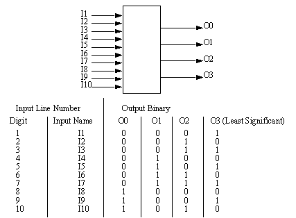
Another test case was examined for a radically different type of planning. In this case it was for the assembly of a digital circuit. The circuit is a simple digital to binary converter. To do this a design was entered, and a new set of rules was developed. In this case the rules used OR gates, and were able to develop all of the gate selections, and connections.
Figure 1.10 A Digital to Binary Converter
Observing the process plan will illustrate that the plan is complete, although the circuit is not efficient in the use of components. One oddity is that while the plan is complete and correct, it is backwards. This is a result of the backward planning approach.
-------- Work Order Sheets ------------
Product: decade_to_binary
OPERATION SUMMARY_SHEET: D_PART - Quantity 1.000000
OP# Operation Description
------------------------------------------
0 Connect gate output 2_INPUT_GATE_5 to output D_OP5
10 Use 2 input OR gate for 2_INPUT_GATE_3 I10
Output is 2_INPUT_GATE_5
20 Use 2 input OR gate for I8 I9
Output is 2_INPUT_GATE_3
OPERATION SUMMARY_SHEET: C_PART - Quantity 1.000000
OP# Operation Description
------------------------------------------
1000 Connect gate output 2_INPUT_GATE_12 to output C_OP12
1010 Use 2 input OR gate for 2_INPUT_GATE_10 I7
Output is 2_INPUT_GATE_12
1020 Use 2 input OR gate for 2_INPUT_GATE_8 I6
Output is 2_INPUT_GATE_10
1030 Use 2 input OR gate for I4 I5
Output is 2_INPUT_GATE_8
OPERATION SUMMARY_SHEET: B_PART - Quantity 1.000000
OP# Operation Description
------------------------------------------
2000 Connect gate output 2_INPUT_GATE_21 to output B_OP21
2010 Use 2 input OR gate for 2_INPUT_GATE_19 I10
Output is 2_INPUT_GATE_21
2020 Use 2 input OR gate for 2_INPUT_GATE_17 I7
Output is 2_INPUT_GATE_19
2030 Use 2 input OR gate for 2_INPUT_GATE_15 I6
Output is 2_INPUT_GATE_17
2040 Use 2 input OR gate for I2 I3
Output is 2_INPUT_GATE_15
OPERATION SUMMARY_SHEET: A_PART - Quantity 1.000000
OP# Operation Description
------------------------------------------
3000 Connect gate output 2_INPUT_GATE_30 to output A_OP30
3010 Use 2 input OR gate for 2_INPUT_GATE_28 I9
Output is 2_INPUT_GATE_30
3020 Use 2 input OR gate for 2_INPUT_GATE_26 I7
Output is 2_INPUT_GATE_28
3030 Use 2 input OR gate for 2_INPUT_GATE_24 I5
Output is 2_INPUT_GATE_26
3040 Use 2 input OR gate for I1 I3
Output is 2_INPUT_GATE_24
OPERATION SUMMARY_SHEET: decade_to_binary_PART - Quantity 1.000000
OP# Operation Description
------------------------------------------
4000 Connect output for D_PART
4010 Connect output for C_PART
4020 Connect output for B_PART
4030 Connect output for A_PART
Figure 1.11 A Process Plan for Circuit Construction
6.0 CONCLUSION
There are a number of available features and items of interest that should be pointed out.
• The feature recognition problem is simplified through the use of a complete design representation, and abstraction with Boolean Algebra.
• Capable of planning for alternate, and new production technologies. This is a benefit of using Boolean algebra that allows a theroetically complete set of description tools.
• Alternative operations are naturally generated during planning. The non-unique nature of Boolean representations ensures alternatives are available.
• The planner can adapt to changes on the factory floor. The ability to replan allows invalid plans to be redone using updated information.
• Human intervention and effort is minimized. The planner, as described, will run without intervention, unless a plan is not found.
• Partial process plans can be generated if the whole plan fails. The planner keeps track of the plan steps it has tried, and these do form a partial plan.
• Process plans can be partially optimized. The techniques allow for selection of plan steps based on cost estimates, and this leads to selection of sub-optimal solutions.
• There is a full breadth of implementations. All of the methods described were developed, and tested, to verify the approach in general.
The current implementation is done in C++, and the core of the planner runs under MS-Dos and UNIX. The time for plan execution is generally a few seconds, up to half a minute for the clothes pin example. The software uses dynamic memory allocation, and has used less than half a megabyte for either of the test cases described here.
The planner described here only uses Boolean reasoning to determine plans, but work being done now will lead to addition of a solid modeller to allow geometrical reasoning. There are also other areas that will require future work. These are,
• connection to a solid modeller to allow geometric reasoning,
• inclusion of variant strategies to reduce replannings,
• connection to other process planner to get more detailed operation lists,
• consideration of fixtures, tools, etc. in the planning stage,
• database lookup - such as that used in the MetCut Database
• exploration of other manufacturing technologies, such as Rapid Prototyping, Chemical machining, Laser machining, EDM, etc.
REFERENCES
[1] Gupta, S., and Turner, J., “Variational Solid Modelling for Tolerance Analysis”, IEEE Computer Graphics and Applications, May 1993, pp. 64-74.
[2] Hoffman, C.M., Geometric and Solid Modelling; An Introduction, Morgan-Kaufmann Publishers Inc., San Mateo, California, 1989.
[3] Jack, H., A Boolean Algebra Approach to High-Level Process Planning, A Ph.D. Thesis presented at the University of Western Ontario, 1994.
[4] Lee, Y.C., Fu, K.S., “Machine Understanding of CSG: Extraction and Unification of Manufacturing Features”, IEEE Computer Graphics and Applications, January 1987, pp. 20-32.
[5] Requicha, A.G., and Rossignac, J.R., “Solid Modelling and Beyond”, IEEE Computer Graphics and Applications, September 1992, pp. 31-44.
