1.5.1 Expert Systems

The most popular approach to recognition is using rules that are based upon human experience. The rules for an expert system are derived by a Knowledge Engineer who consults human experts. In general the rules are of the ‘if <conditions> then <action>’ form. As these rules are applied to a known set of facts, new facts are found. Most researchers use these rules to examine geometrical and manufacturing facts, in order to recognize manufacturing features. Some of the classic systems are excellent examples of rule based reasoning, such as GARI [Descotte and Latombe, 1984], TOM [Matsushima et. al., 1982], EXCAP [Davies and Darbyshire, 1984], XPLAN [Alting, et. al., 1988], etc.

The expert system approach is well suited to designs stored symbolically. Other expert system approaches use Frame based reasoning or Decision Tables. It is quite common to augment data in a frame with connectivity (derived from B-Rep models) to other faces and features to facilitate symbolic condition testing. A good overview of expert system use in CAPP is available in Alting and Zhang [1988].

1.5.2 Syntactic Pattern Recognition

By encoding the geometry of a part using a set of grammatical symbols, an abstract expression may be formulated. A matching process may then be performed between the syntax of the derived grammatical expressions and grammatical syntaxes of known features. An example of this could be a representation of a sheet metal part. The part is described with line geometry, as pictured in Figure 1.4 Syntactic Pattern Representation of a Sheet Metal Design. A basic set of grammars are define for the shape. These are then applied to the shape to obtain a code for use in pattern matching. Here we see code for the part begins at the top left corner, and works around in a clockwise direction.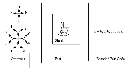

Kusiak [1991] summarizes the process of Syntactic Pattern Recognition as three distinct stages. Initially, an input string (w = a1, a2, ..., an) and an extended context-free grammar (G = (Vn, Vt, P, S)), form the input to a schema. The context-free grammar is composed of,

Vn set of input symbols described in the input string

Vt set of symbols which will comprise the solution

P a set of production rules which will transform the input string

S (containing symbols Vn) into an output string G which contains

symbols only in Vt

S starting set, as w above.

The syntactic pattern recognition approach is used by Liu and Srinivasan [1984] to select machine tools for manufacturing parts.

1.5.3 State Transition Diagrams

Whereas the Syntactic Pattern Recognition was based upon a large set of grammar, the State Transition approach uses a binary operator. When moving between previous features there are relative changes from concave to convex. These changes are marked with a state of 1 or 0 respectively. The profile of a part may be converted to a string, similar to the method shown in Figure 1.4 Syntactic Pattern Representation of a Sheet Metal Design. This is then fed to an automata which uses state transition diagrams to classify features. A State Transition Diagram may be seen in Figure 1.5 A State Transition Diagram for Feature Recognition. This example begins at the top left-hand corner, then proceeds in a clockwise direction. The only ‘1’ in the sequence represents the concave transition near the top right-hand corner.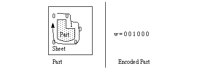

The code for a part is then examined for recognized sequences (sub-strings). For example, if the shape encoded is for a power screw thread, the code would contain a string such as ‘......0011001100110011...’ (This is because of the square thread). Therefore, recognizing the string contains a power screw thread, the planner would be able to select the appropriate tooling, and cutting operation.

1.5.4 Graph-Based Approach

While Syntactic Pattern Recognition and State Transition Diagrams are best suited to planar parts and rotated profiles, graph-based approaches are suited to full three dimensional parts. Kusiak [1991] describes the form of the graph as G = (N, A, T) where,

N represents nodes in the graph

A represents arcs between nodes

T represents attributes assigned to the arcs

This basic method involves capturing the design geometry in the form of a graph. The graph is then examined for patterns that match known features.

Joshi and Chang [1988] and Joshi, Vissa and Chang [1988] developed the Attribute Adjacency Graph (AAG). Each face is represented as a node. The arcs are the edges, or adjacency. The attribute of the arc is assigned a value of 0 or 1 depending upon a concave or convex transition, respectively. They then recognize features with algorithms and rules. The algorithms find candidates for indented features by examining the concavity of points. When potential features have been identified, the AAG is examined with production rules to compare features to feature graphs. They also deal with interacting features and there are three cases they discuss. The first is nested features, such as a pocket milled inside a pocket. In this mode, features are identified and then cut out of the AAG. The next case is intersecting features, such as two slots cut to cross each other. To detect this condition, virtual surfaces are created, then the features reexamined. Finally, when the forms of features interact, such as two stepped slots, the feature is dealt with by using virtual pockets. The important feature of these methods is the creation (or destruction) of new subvolumes to clarify feature details, and therefore simplify recognition. Their work was implemented for machined parts with indented features.

Sakurai and Gossard [1988] have an interactive system which the user uses to identify significant faces in a feature by selecting faces on a B-Rep model. They can search a B-Rep model to identify subsets that correspond to known features. deFloriani[1987] categorizes recognized features into depressions, protrusions, and holes from a B-Rep Model. The simple features are then grouped into compound features. The final model is a generalized edge face graph.

In general the syntactic pattern recognition, state transition diagrams, and graph based approaches are all suited to models that have some form of 2D or 3D B-Rep model. These methods can recognize features in an object, unless they overlap, but they are not able to reason past that stage.

1.5.5 Constructive Solids Approach

A very limited number of methods have examined the use of Constructive Solids Geometry (CSG), also known as the Set Theoretic method. The CSG method uses primitive volumes, and then performs additions, joins, and removes between them to form more complex objects. Eventually complex geometries can be built up.

In some early work in the area of solid modelling, Woo [1977] developed a CSG based process planning method. His system allows design, process planning and then milling of cavities into parts. At the front end of the system is a solid modeler called CARVD. The system has two operations, ADD and REMOVE (a sub-set of the full CSG operations). The system puts the design into a nested algebraic expression, which is searched for cavity patterns. This search progresses from the most nested term to the least. The search involves determining ‘hooks’ between the terms in the algebraic expression. The system then uses interpretive rules (in the form of semantic nets) to match these to features (see Figure 1.6 The CARVD Method of Feature Recognition).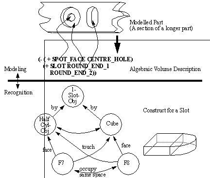

(Adapted from [Woo, 1977])

After a feature is chosen, the NC code is generated. The procedure of selecting an NC tool path involves an approach direction for the feature. The method of NC code generation is highly specific to cavity milling. This method of casting the expression in a nested equation form is similar to the representation used in this thesis.

Woodwark [1988] philosophizes about CSG approaches to Feature Recognition. He identifies the non-uniqueness of the CSG model as one of the faults of the method. He argued that the non-uniqueness of the method makes search spaces much larger, and therefore harder to search and prune. As a result, he suggested three ways to overcome these problems.

• Restrict the domain of the model, by restricting the range of primitives and orientations that they may assume (used in the work by Woo [1977]).

• To restrict the ways in which primitives may interact spatially.

• To restrict the allowable forms of set theoretic expressions which define the model.

By limiting the complexity of the model, it is possible to limit the complexity of the designs is also limited. Woodwark also suggests matching to shape templates. This method involves using feature templates that are applied to local parts of the CSG model. This is similar to traditional pattern matching, except that it is localized for specific features to save search time. He claims this method can fail when two or more features interact, thus causing the feature matching to be inconclusive.

The final approach proposed by Woodwark is a hybrid CSG and Boundary Representation. He discusses adding geometrical boundary information to the set theoretic model. In this way the benefits of CSG are maintained, while making the actual geometry available for geometrical reasoning.

Work has been done by a number of authors to recognize features using CSG pattern recognition. Kakazu and Okino [1984] developed a method for converting a set theoretic representation of a part into a canonical form, and then a pattern recognition approach was used to find a Group Technology code. Other work for manipulating CSG trees was done by Goldfeather et. al. [1986] who developed the CSG tree into a normal form for faster computer graphics. Lee and Jea [1988] also developed a method for moving single nodes up through a CSG tree for the purpose of eventually developing a system that recognizes CSG features recognizing features. They only provided a brief description of how a feature recognition algorithm would work.

1.5.6 Decomposition

The method of the previous section is successful, but assumes that the CSG operations are all subtractions of machined features. But, this is not always the case, sometimes a larger stock shape must be selected before features can be recognized. After the stock is selected, solid models can be decomposed into smaller subvolumes through iterative methods. These subvolumes may then be examined by a feature recognition stage. There are common methods often used for this technique. These methods are often based on some sort of differencing operation to derive sub-volumes.

1.5.6.2 - Alternating Sum of Volumes (ASV)

A method of overcoming the non-unique properties of CSG representations has been suggested by Tang and Woo [1991a,b]. Their papers discuss a method of decomposing a solid into a set of convex solids. This is done using an iterative method of covering an existing part with a convex hull. The hull then has the basis part subtracted. The same operation is continued on the remaining solid until there is no solid left. The result is a set of volumes that may be resolved into a set of removable volumes. An example from their paper is shown in Figure 1.7 The Alternating Sum of Volumes (ASV). In the example, the part goes through a number of iterations to identify the primitive geometry components. At the bottom of the figure the primitives are collected and then simplified to material removal only. The very bottom of the figure shows a set of primitive shapes that may be removed (H1’ and H3) from the stock (H0) to produce the part.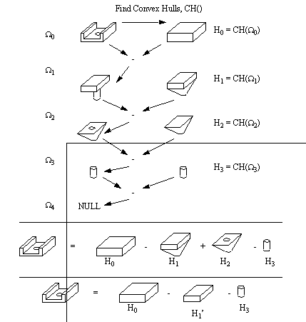

 

Figure 1.7 The Alternating Sum of Volumes (ASV)

(the figures depicted here are not to scale for clarity) [Tang and Woo, 1991a,b]

Although this method will determine a set of machinable features, it has some problems which the authors also identified. Tang and Woo [1991b] refer to these problems as nonconvergence. And, considering that this method is iterative, the algorithm would continue indefinitely, as shown in Figure 1.8 An Example of a Nonconvergent ASV. The have proposed an algorithm to check for nonconvergence based upon strong, weak, and internal hull vertices. They present a set of algorithms, in pseudocode, that deal with a Boundary Representation. These algorithms have also been developed to deal with non-manifold edges and vertices.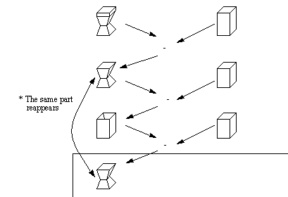

 

Figure 1.8 An Example of a Nonconvergent ASV