Jack, H., “System Modeling and Control for Mechanical Engineers”, ASEE Annual Meeting, Montreal, Quebec, June 2002.

Abstract

Traditional courses in systems modeling focus on linear analysis techniques for systems using Laplace transforms. This method is highly effective for electrical engineering students who will make use of these techniques throughout their studies. For various reasons, such as non-linearity, Laplace transforms are used less frequently in mechanical engineering. In recognition of this difference, the Dynamic Systems Modeling and Control course (EGR 345) at Grand Valley State University was redesigned.

EGR 345 examines systems that contain translational, rotational and electrical components, as well as permanent magnet DC motors. These systems are modeled with differential equations. The students are shown how to solve these systems of equations using explicit integration, numerical integration, and recognition of the canonical forms. Students are then shown how to manipulate equations containing the differential operator, and how to put these into transfer function form. Once in this form it is possible to utilize most of the techniques of classical linear control, such as block diagrams, Bode plots and root-locus diagrams.

The course includes a major laboratory component. In the first half of the semester the laboratories focus on modeling physical components. The models can then be used to predict the responses of systems to given inputs. As the semester progresses the labs transition to using industrial motor controllers to reinforce the value of the course material.

The paper describes the course in detail, including a custom written text book available on the course web page ( http://claymore.engineer.gvsu.edu/courses.html) .

Introduction

At Grand Valley State University (GVSU) all junior Mechanical and Manufacturing engineering students take EGR 345, Dynamic Systems Modeling and Control. Originally this course followed a very traditional approach using Laplace transforms to analyze lumped parameter linear systems. When the students completed the course they were able to analyze single input, single output linear systems using Laplace transforms, by integrating first and second order differential equations, and using numerical methods. The topics covered in the old version of the course are listed below.

• Introduction

• Translation

• State variable form

• Rotation

• Electrical systems

• First and second order systems and integration

• Laplace transforms

• Transfer functions

• Block diagrams

• Feedback control systems, Bode plots and root-locus diagrams

The textbook used for the older version of the course was written by Close and Frederick [1]. It covers the analysis of systems using differential equations and numerical methods, but quickly goes on to use Laplacian techniques. This approach is sensible for students in Electrical engineering. They are exposed to these topics in many other courses, thus allowing the material to be quickly reviewed before moving into advanced topics such as system analysis and controls. In addition, electrical systems components are generally easy to linearize, thus allowing the used of Laplace transforms. By contrast, Mechanical engineering students are more likely to use calculus and numerical methods to analyze non-linear systems. They are unlikely to be exposed to Laplace transforms in any other engineering courses, before or after the systems modeling course. A large amount of time is consumed presenting the transforms for the first time in the modeling course, and the material is not reinforced in subsequent courses. As a result most Mechanical engineering students are overwhelmed by a rushed treatment of transforms and controls in a single course. This does not have to be the case.

After significant reflection about the challenges in trying to teach systems modeling it was decided to reform the course to be more suitable to Mechanical (and Manufacturing) engineers. In particular the Laplace transform was removed. This freed time to increase the coverage of differential equation solutions and numerical methods. Counter to expectations, removing Laplace transforms did not require the elimination of techniques such as Bode plots and root-locus diagrams. A side benefit of this approach is that it allowed more time to address math deficiencies. In particular, all students had completed a four course calculus sequence, but many still had basic problems [4]. The course was also enhanced by adding labs and tutorials that used industrial equipment to emphasize the theory in practical applications. This also helped to fulfill the mission of the School of Engineering by helping to meet the needs of local industry.

Maturing Beyond Linear Systems

Historically most system modeling and control courses are rooted in the techniques of Electrical engineering. For example, the book used previously [1] was written by an Electrical engineer, and the author of this paper has a degree in Electrical engineering. As a result the techniques for analysis tend to examine lumped parameter linear systems with Laplace transforms. For students outside Electrical engineering this is unnecessary, and displaces other useful techniques from already full curriculums. Consider the very fundamental case of a falling mass experiencing aerodynamic drag which results in an equation of the form,

.

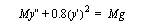The velocity squared term will prevent the equation from being converted to a transfer function, and prevent system analysis with Laplacian methods. However, this system can be integrated as a separable equation, or integrated numerically by converting it to a state equation.

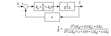
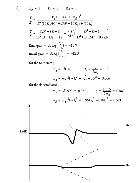
Eliminating the Laplace transform doesn’t eliminate the ability to use many analysis techniques associated with the Laplace transform. The differential operator can be manipulated algebraically, and in many ways is analogous to the Laplacian ‘s’. This can be seen in texts [2][3] that use the differential operator. An example is shown in Appendix A. The block diagram shows a negative feedback system using a PID controller for error compensation. The ‘D’ is an alternate notation for the differential operator ‘d/dt’. If the system starts at rest the ‘D’ could be replaced with the Laplace ‘s’. In this case the system block diagram is simplified, a root-locus analysis is done, a Bode plot constructed, and the system response is found (a zero response in this case) by solving the differential equation.

A New Course

The new course format was offered successfully for the first time in the fall of 2001. The list of course topics is given below.

1. Introduction and math review

2. Translation

3. Calculus and differential equations

4. Numerical methods

5. Rotation

6. Input-output equations

7. Circuits

8. Feedback controllers

9. Fourier and root-locus analysis

10. Converting between analog and digital

11. Sensors

12. Actuators

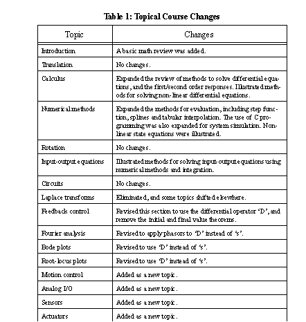
The general sequence of topics is similar to those of the old offerings. The primary difference emerges in the mathematical emphasis on specific topics as shown in Table 1. This new format also allowed the introduction of new topics that are also considered important, such as motion control, sensors and actuators.

At the completion of the course students were able to analyze a wide variety of systems. Although they were not familiar with Laplacian techniques they were still able to analyze linear systems with explicit, or numerical integration. They were also able to deal comfortably with non-linear systems. This format also improves their proficiency with techniques that are applicable in subsequent math intensive course, such as fluids.

Using Industrial Hardware

An Electrical engineering student taking a controls course can design and build many examples of feedback amplifier systems. However Mechanical engineering students are often challenged by a lack of context when studying control systems. To overcome this a number of tutorials and laboratories were added that involved industrial control equipment and sensors.

Throughout the laboratory sequence industrial sensors were used for data collection. Towards the end of the laboratory sequences the labs turned to the use of motors and controllers. In these labs the students altered controller parameters and gains. The servo and variable frequency motors all allowed the students to modify PID controller parameters. As a result the students had been given many opportunities to use systems that were under/over damped, and relate these behaviors to controller gains. A list of the laboratory exercises are given below.

1. Web page creation and Mathcad tutorial/review

2. Computer based data collection with Labview

3. Sensors (accelerometers, potentiometers, ultrasonic, etc.)

4. Permanent magnet DC motor modeling

5. Proportional feedback controller

6. Spring and damper modeling

7. Torsional oscillation of a mass on a thin rod

8. Servo control systems - Allen Bradley Ultra 100 drives

9. Servo control systems and programming in C - Allen Bradley Ultra 5000 drives

10. Op-amp audio filters

11. Stepper motor controllers

12. Variable frequency drives - Allen Bradley 161 series

The result of the laboratory sequence was that students were familiar with industrial equipment and how it was related to the theory covered in the lectures. The connection between the theory and actual equipment reduced the resistance to the theory that students previously exhibited.

Conclusion

The revised format of the course has helped focus on the mathematical skills that are useful to Mechanical engineers. The removal of Laplace transforms does not prevent the students from evaluating linear systems. However the emphasis on numerical techniques enables them to analyze more complex systems. In addition, the time spent reviewing and applying calculus techniques learned previously also improves their mathematical preparation for future courses.

A number of indicators speak to the success of the course. In particular the student attitude was notably better at the end of the new course format. The final exam scores also rose to ‘C’ in the new format from ‘D’ for the old. The results of this updated course will be reviewed rigorously when the students who took it for the first time in the fall of 2001, return for their next regular academic semester in the summer of 2002.

References

[1] Close, C., and Frederick, D., “Modeling and Analysis of Dynamic Systems”, Second Edition, Wiley, 1995.

[2] Raven, F, “Automatic Control Engineering”, Fifth Edition, McGraw-Hill, 1995.

[3] Jack, H., “ Dynamic System Modeling and Control”, http://claymore.engineer.gvsu.edu/~jackh/books.html, 2002.

[4] Adamczyk, B., Reffeor, W. and Jack, H., “Math Literacy and Proficiency in Engineering Students”, ASEE Annual Conference Proceedings, 2002.

Biography

Hugh Jack is an Assistant Professor in the Padnos School of Engineering at Grand Valley State University. He has been teaching there since 1996 in the areas of manufacturing and controls. His research areas include, process planning, robotics and rapids prototyping. He previously taught at Ryerson Polytechnic university for 3 years. He holds a Bachelors in electrical engineering, and Masters and Doctorate in Mechanical Engineering from the University of Western Ontario.

Appendix A - A Problem Example

A feedback control system is shown below. The system incorporates a PID controller. The closed loop transfer function is given.

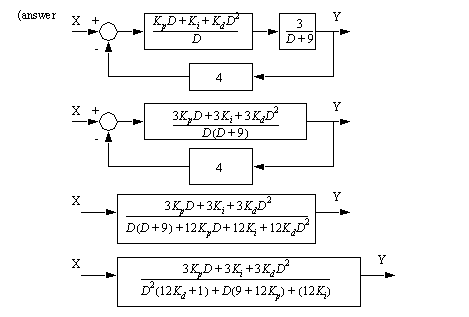
a) Verify the close loop controller function given.

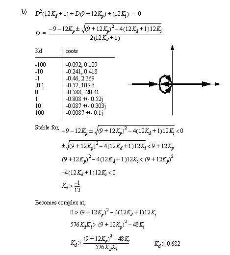
b) Draw a root locus plot for the controller if Kp=1 and Ki=1. Identify any values of Kd that would leave the system unstable.

c) Draw a Bode plot for the feedback system if Kd=Kp=Ki=1.

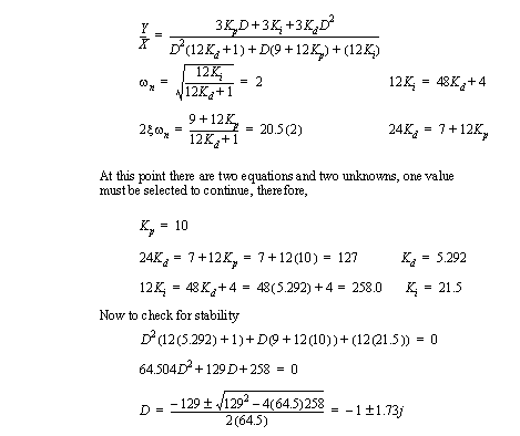
d) Select controller values that will result in a natural frequency of 2 rad/sec and damping coefficient of 0.5. Verify that the controller will be stable.

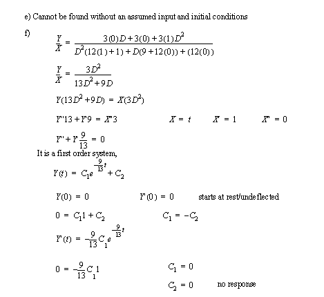
e) For the parameters found in the last step can the initial values be found?

f) If the values of Kd=1 and Ki=Kp=0, find the response to a unit ramp input as a function of time.