1. A REVIEW OF ROBOT MOTION PLANNING
2.1 Introduction:
Robots are primarily designed to manipulate objects in space. This involves some form of motion through space. Choosing the motion involves a large number of problems. These problems typically begin at the task level, where task requirements are generated. A motion is planned, to satisfy the task requirements, after the task requirements are specified. The motion planning problem has a few distinct elements.
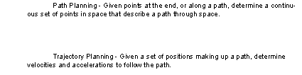
Motion planners must determine trajectories in space, along unspecified paths. A basic way to achieve this is to use a Path Planner to determine a path. A Trajectory Planner may then use the path to determine the trajectories that will move the robot through space.
If a path is not completely specified, a Path Planner may be used. If a complete Path Plan is available, a Trajectory Planner may be used to determine the optimal motion along the path. After motion on a path has been determined, the motion may be translated into control variables. Each of these planners will consider particular constraints, based upon the problems they are solving.
The concepts of the various problems may be put in a mathematical context,
Figure 2.1: The Problem Hierarchy of Robot Motion Planning
The mathematical formulations are general, and may be interpreted in any number of ways. As the diagram illustrates, each of the problems may be defined as a sub-set, or a super-set of the other.
2.2 Trajectory and Path Planning:
Brady et. al. [1982] described the Trajectory Planning problem as, “The process of computing a sequence of positions, velocities and accelerations is called trajectory planning”. Thus, the time evolution of the robot states (i.e., motion) is the basis of the problem. A path is commonly required for Trajectory Planning. This path becomes a constraint for the trajectory planner, and it must be generated separately by the Path Planner.
The path planner is responsible for generating a continuous set of positions in space, which the manipulator may move along (i.e., a continuous set of robot states). Thus, this planner is concerned with the spatial aspects of this problem. This problem may involve constraints like collisions, path endpoints and, kinematic constraints of the robot.
Some researchers have integrated these functions, while others have kept them separate. The approach is often related to how the path is represented.
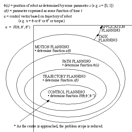
Figure 2.2: An illustration of a Path Plan vs. Trajectory Plan
2.3 Robot Path Description:
A robot path in space can be expressed in many ways. But all paths require that robot positions be mathematically described, as they evolve through a motion. This involves two problems, representing positions and transformation of positions along the path.
Robot positions may be described in many ways. The robot positions may be expressed in terms of the position of the end effector, in Cartesian space. The robot position may also be described as a joint configuration (joint angles in this thesis). Other methods exist, but the two above are the most common.
Via points in Cartesian space are often used to define a path. These are sample points along a path, which the manipulator end effector should pass through. For example, a set of via points may be used to construct a spline in space, which the end effector must follow. Representation of paths in space has advantages when dealing with physical objects, and tasks. Although, paths can be hard to convert to robot joint coordinates when they are described in Cartesian space it is easy to consider obstacles.
Joint coordinates are also used for path description. As before, a spline may be fitted to a path described with via points in joint coordinates. Paths expressed in joint coordinates can be advantageous for path, and trajectory planning. The joint positions, velocities and accelerations may be obtained directly from this representation, thus easing algebraic complexity. Joint coordinate representation encounters problems when real space constraints must be considered. For example it is very hard to map an obstacle into joint space for collision detection problems.
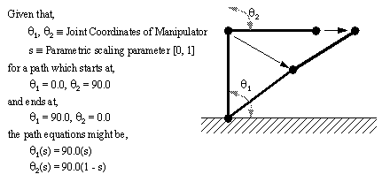
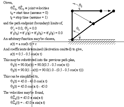
The robot positions must be described as they evolve along the path. The given path representation may contain positions at all, some, or none of the points on the path. If the path description is incomplete, some method must be used to ‘fill-in’ the incomplete sections on the path. Thus, paths are often modelled with continuous, mathematical functions. A robot is shown below with a simply formulated, example path. Initially, this path is described with motion endpoints, in joint coordinates. A simple path is then suggested between start and goal configurations.
Figure 2.3: A Sample Robot Path (joint interpolated)
Note that the path has no time scale associated with it, this will be done later in the trajectory planning stage. Also note that, the functions are very simple, but something more complex could have been used.
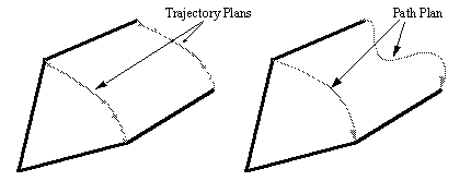
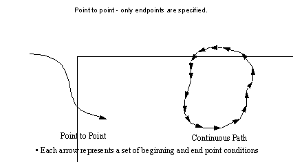
The representation of a path plan also requires other considerations. Usually the path will be point to point (i.e., from a current position to some goal position). Paths may also be continuous, for example when robots are used for painting, welding, and gluing. The continuous path tends to have motion requirements for various path segments. Point to point is easier to model, because the endpoints for the path are well defined and fixed.
Figure 2.4: Point to Point and Continuous Paths
The description of the path between endpoints is also important. A path plan should have continuous position vectors between motion endpoints, to ease trajectory planning. Sharp corners on the path may also cause planning problems.
2.4 Robot Path and Trajectory Description:
A trajectory is a description of the robot motion through space. Paths are used as position constraints in space, with no implied time relationship. Trajectory planning is the task of associating time with the path. As before, the path positions may be described in several ways, for example joint coordinates. The set of joint coordinates may be connected with splines through joint space.
A trajectory planner is highly specific to the path plan. One example could be a path that is expressed in splines with parametric scales. The trajectory planner must then derive a parametric time function. Once time has been associated with positions, the velocities and accelerations may be found.
A simple example of Trajectory Planning is shown below, using the path descriptions derived in the previous section.
Figure 2.5: A Sample Trajectory Plan (extension of the sample path in Figure 2.3)
The reader should note that the function chosen for ‘s(t)’ is simple, and could have been much more complex. The coefficients for this function can also be derived quite simply. Although this derivation is somewhat ad hoc, it results in a simple set of motion equations.
2.5 Motion Planning:
Motion planning assumes that the path planner and the trajectory planner are combined somehow. This approach creates some fundamental differences when attempting to make optimal use of robot properties.
For example, some researchers combine path planning, and trajectory planning, and directly determine the best paths. For example, one idea involves the use of a Switching Point. A Torque Switching Point is best understood if one thinks of it as the point midway along a path when the robot must reverse acceleration, and begin deceleration. As the switching point is tested at different times on the path, the path shape, and the path trajectories all change. This approach can be very powerful.
Other researchers attempt to represent path and trajectories at the same time. By altering the shape of the motion representation, they directly alter the positions, velocities and accelerations. This approach is often used when attempting to obtain paths with some form of optimization (as is done in this thesis).
2.6 Optimal Motion Planning:
There are an infinite number of path and trajectory plans between two points [Dlabka, Held & Zhang 1988]. Therefore, a description of a trajectory and path is somewhat arbitrary. When deciding upon a robot motion, there must be some objective. Common objectives are,
• minimum time,
• minimum energy, or
• shortest path length.
These objectives are usually constrained. Common constraints are,
• actuator position limits,
• actuator velocity limits,
• actuator acceleration limits,
• actuator jerk limits,
• actuator torque limits,
• kinematics (e.g., outside robot reach),
• collisions and,
• task constraints.
The motion planning problem may be solved to make the solution globally optimal, locally optimal, sub-optimal, or non-optimal.
A non-optimal motion is one that is determined with little or no attempt to minimize some objective. These are not very practical, and not very common. Even when a motion is manually entered on an industrial robot, the programmer will attempt to reduce motion time. When a motion has been manually programmed, the controller will often find a sub-optimal motion between programmed points.
Sub-optimal methods do not require much complexity in modelling and computation. These methods tend to find optimal (or sub-optimal) solutions for the next action. An example would be an optimal control scheme. The global solution is often sub-optimal when all the locally optimal solutions are strung together.
Locally optimal methods tend to find optimal solutions to sub-problems. An example of this sort of problem would begin with a Path Planner that finds an optimal path. An Optimal Trajectory Plan is then generated for this path. Even though both the Trajectory and Path Plans are optimal, their combination is not likely to provide the optimum motion. This can be restated as, an optimal path and trajectory do not indicate globally optimal motion. Globally Optimal motion planners find the best path plan and trajectory plan combination.
Global motion planning often results in an effect where the optimality of the solution is traded off with computation time. The problem complexity grows with the selection of objectives, and constraints. Thus, objectives and constraints must be chosen carefully.
The choice of objectives and constraints is based upon the chosen task of the robot. If the robot is in an industrial setting, time may be very important, thus time should be the objective. If the robot is not a bottle neck on an assembly line then least energy may be more efficient. Shortest path approximations are usually done as an approximation for minimum time. Alternately, the selection of constraints are often predetermined, but some simplifications may be made to speed computation time.
In closing it should be noted that optimization is not the only way to obtain better paths. Miller et. al. [1990] proposed a novel approach that avoids the classical optimization approach. They developed a method for iteratively improving a path, every time it is traversed. This path will eventually converge to a very good match. But, since the method is best for paths repeated thousands of times, it does not offer much improvement over off-line programming methods.
2.7 Kinematic Motion Planning:
Kinematic motion planning involves the planning of motion through space, while not violating some combination of position, velocity, acceleration, and jerk constraints. These kinematic constraints are often determined by actuator limits like torque and velocity. Abstract limits like torque can be converted into acceleration limits, based on position and velocity. As a result of the non-linear characteristics (dynamics) of the manipulator, kinematic limits vary over the workspace.
The limits can be determined and used in one of two ways. The local kinematic limits may be estimated in a region, by evaluating the dynamics locally. The local estimation of kinematic limits may be used for local motion planning.
The other approach is to find the weakest configurations for the robot. For example, to find the maximum acceleration for an industrial manipulator, the robot could be moved throughout the workspace with a high acceleration limit. If the robot is unable to maintain that acceleration limit, the acceleration limit is lowered. This is continued until the acceleration limit is maintained for all motions. This may be used to determine acceleration limits (valid for all configurations) at the cost of reduced performance. The velocity limits of a robot are an inherent property of the actuators that drive the arm.
Some advantages come from using global kinematic limit values. Using global velocity and acceleration limits, ensures that the actuator limits will not be violated. Since the velocity and acceleration limits ensure that actuator limits will not be violated for any path, the coupling of actuator limits has been eliminated. Because the actuators are “uncoupled”, they may be considered separately. Therefore, traditional linear control methods may be used. Current commercial systems use these methods [CRS Plus Inc., 1987], but the approximations lead to a significant reduction in potential performance, and non-uniform control response.
2.8 Dynamic Motion Planning:
Dynamic motion planning involves motion through space, while avoiding dynamic constraints. The dynamic constraints are usually in the form of torque and force limits. This method always requires some model of the manipulator dynamics. This model may be explicit with a numerical integration, or approximate with a discrete estimation.
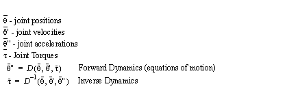
If position, velocity and acceleration are provided, the inverse dynamics of the manipulator may be used to find the instantaneous joint torques. If the position, velocity and torque are provided, the forward dynamic equations may be used to determine instantaneous acceleration.
If a torque is applied for some time, then the forward dynamics equation must be integrated to find the effect of torque on position and velocity. If the position, velocity, and acceleration are applied, then the inverse dynamics may be integrated over some time period to find the path energy. As an alternative to the integration, some discrete approximate models have been devised.
Neuman and Tourassis [1985] have devised a discrete approximation for robot dynamics, based on the Lagrange-Euler formulation. Their model produces near real-time approximations of robot dynamics. Their method is not as accurate as the adaptive time step Runge-Kutta integration of dynamics equations (used here), but it is more accurate than many other methods.
One assumption that is often made in Dynamic Motion Planning is that the joint torque maximum limits are fixed constants. But, these may vary if the actuators are non-linear, or there is energy loss in the torque/force transmission. As a result of a ‘no-loss’ assumptions Yamamoto and Mohri [1989] state, “By the Maximum Principle we know that the solution for the time optimal control problem in which a control term appears linearly in the dynamic equation is of a bang-bang type.” If the reader looks ahead they will notice that the case used in this thesis has the joint torque appearing linearly in the dynamics equations (see figures 5.8, 5.9, 5.10). Thus, the optimal control type is assumed to be bang-bang for time optimal control.
2.9 Trajectory Planning:
Once a path has been determined, a plan of how to traverse it may be generated. A path in space may be characterized by many methods, as mentioned before. All the trajectory planners must take the path description and generate a trajectory plan for the path.
A common trajectory planning method is to use splines in Cartesian space to represent end effector position [Fu, et. al., 1987][Shahinpoor, 1987][Craig, 1986]. At each point on the spline, the end effector position, velocity and acceleration may be determined. The inverse Jacobian of the manipulator may be used to find the joint velocities and accelerations. Then, the inverse dynamics may be used to find the required joint torques. Adjusting the time scale of the spline will allow the manipulation of the trajectory plan. If the time scale is adjusted appropriately, the optimal trajectory plan may be obtained [Bobrow, et. al., 1983].
Trajectory planning may also be done by more established approaches. At Present, Feedback Control systems are used to track trajectories or paths that have been planned. This is a preferred mode of operation, but they may also serve a dual purpose by moving over long paths, and thus acting as path generators, instead of as path followers.
Current robots will typically use a simple feedback controller to control position [Spong and Vidyasagar 1989]. This approach will not provide the optimal trajectory, and thus robotics researchers have looked towards more sophisticated non-linear control methods.
Adaptive, and model based controllers have formed the basis for many locally optimal trajectory planners. These controllers allow their control laws to adapt as the path is traversed. Thus, these methods are not simple and do require sophisticated models, which may not adapt to payloads, and are highly particular to one robot. As stated before, Kuntze [1988] suggests that hardware requirements for sampling speed, processing speed and memory volume are very demanding on model based algorithms. He also says that current complex robot models (for control) require sophisticated computers, experimentation and modelling procedures. Miller et. al., [1990] also explain that the use of adaptive controllers have problems based on the high computational requirements for real time parameter identification. Their sensitivity to noise and numerical precision will grow as the number of system variables increase.
2.10 Optimal Trajectory Planning:
As discussed before, bang-bang control is time optimal for a motion plan. Trajectory plans are often formed while observing velocity, acceleration, jerk, and torque limits. For example, Spong & Vidyasagar [1988] discuss least time trajectories using velocity profiles. Other approaches have used more elegant approaches to the Trajectory Planning Problem.
Kim and Shin [1985] describe their method for finding an optimal trajectory plan for a path described with a set of straight line segments in space. They approximate the maximum velocity and accelerations for each path based on the maximum torque for the joint segment. Thus, when following the line segment, the robot moves at maximum velocity. They also propose a method to ‘round’ the sharp corners on the path. This means that there is no stop/start at the straight path segment endpoints. This method could be replaced by one that does not assume straight path segments in space.
Flash and Potts [1985] discuss a method for optimizing a path described with a set of via points. They use Neuman and Tourasis’ [1985] discrete dynamic model of the robot with a linear programming approach, to choose a set of constant accelerations between each pair of via points. Tan and Potts [1988] have extended the work done by Flash and Potts [1985] by using the iterative method of look-up programming to refine the trajectories, and by adding dynamics constraints for a 2 degree of freedom robot. In a second paper by Tan and Potts [1989] they extend their work to a full 6 degree of freedom Stanford arm manipulator.
Another method is presented by Ozaki, Yamamoto and Mohri [1987] who propose a method in which a path is represented with a B-spline in Cartesian space. The trajectory plan is improved by shifting the control points of the B-Spline function. This optimizes the path by making subtle refinements.
An exact algorithm has been proposed and discussed by Bobrow et. al.[1983, 1985], and Bobrow [1988]. Bobrow has been able to find optimal trajectory plans for end effector paths in cartesian space. He reformulates the dynamic equations using the path in space, and the actuator torque limits. The modified dynamic equations may then be used to find the maximum acceleration of the end effector as a result of a specific joint torque. The effect of each joint is considered, and the dominant joint is chosen to be the one with the most restrictions on end effector acceleration. An algorithm is then used to determine switching points for the optimal path, based on these limits. In Bobrow [1988], collision avoidance is considered as well.
Shin and McKay [1985] have suggested an improved, more rigorous approach to Bobrow’s algorithm [Bobrow et. al., 1983] for finding optimal paths. Their work revealed that Bobrow’s algorithm might not be able to find the problem solution sometimes.
2.11 Path Planning
There are two types of robot paths, Point to Point, and Continuous [Dlabka, Held & Zhang, 1988]. Continuous paths are typically not issues for path planning researchers. These paths are usually dealt with by the task planner, which will rearrange the task and robot spatial parameters, and produce a highly constrained paths. These paths will then be passed directly to the trajectory planner that will adjust the velocity profiles [Dlabka, Held & Zhang, 1988]. Point to point, and underconstrained, paths must be dealt with by the path planner.
Point to point path planning involves moving a manipulator between a start and stop configuration. There are an infinite number of paths that may be followed. Therefore, some of the optimization criterion might be used for choosing a path. Typical objectives are minimum time, shortest path, least energy [Vukobratovic and Kircanski, 1982], and proximity to obstacles [Espiau and Boulic, 1986]. Typical constraints are collision avoidance, moving obstacles [Lee and Chien, 1987], robot coordination [Suh and Shin, 1989] and task constraints.
Task constraints describe the boundary conditions for the robot motion. Usually they are robot start and goal positions. Redundant manipulators may add a degree of complexity to the problem by allowing an infinite number of solutions at the boundary (start/stop) points as well. A typical redundant manipulator may have seven degrees of freedom, or more, and thus has an infinite number of configurations to reach some points in the work space.
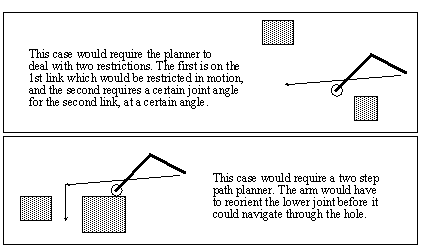
Collision avoidance is commonly called Geometric Path Planning. This involves planning a path through space, which avoids geometric constraints on the path. This is generally done by creating a map of the geometrical properties of space which may, or may not, be a direct representation of space. An algorithm is then typically used to find a path through this map. Examples of this are tessellation [Saher and Hollerbach, 1985], configuration space [Lozano-Perez, 1983], occupation maps, etc. These methods tend to explode exponentially with problem complexity, and are generally hard to convert from space to robot configurations. Two problems are shown below to illustrate two dimensional path collision avoidance problems.
Figure 2.6: Examples of Geometric Path Planning Problems
2.12 Optimal Path Planning
To consider the Optimal Path Planning Problem in more detail, we must iterate some of the obvious points, in rather simple terms. A Path plan involves moving a manipulator between a start and stop configuration. There are an infinite number of paths that may be followed between these points. The infinite number of paths means that some paths will be judged better than others. The measure of optimality for a path can be based on several factors. The most common objective is shortest path. These optimal paths also experience the constraints mentioned in the previous section: obstacle constraints, robot cooperation, moving objects, and task constraints.
Path planners are commonly based on Optimal Geometric Paths. One approach to representing these paths is with spatial maps, and representations. Some techniques that have been used are Swept Volume [Lozano-Perez and Wesley, 1979], Generalized cones [Brooks, 1983a], Freeways [Brook, 1983b], Oct-trees [Soetadji, 1986], Voronoi Diagrams [Takehashi and Schilling, 1989], Potential Fields [Park, 1984][Khosla and Volpe, 1988], and V-graphs [Kant and Zucker, 1988]. Other methods attempt to transform space to simplify calculations. Some examples of these are configuration space [Lozano-Perez, 1979, 1983], and Configuration Joint Space [Red and Truong-Cao, 1985].
2.13 Optimal Motion Planning:
Optimal motion planning is an integrated combination of path and trajectory planning. There are some motion planners that cannot be distinctly divided into path and trajectory planners, these are described in this section. The methods in this section are based on the same objectives, and constraints which were of interest in previous sections.
Buchal [1989] discusses an approach to the motion planning problem in which the path is initially described as a set of points, all equally spaced in time. These points are then manipulated (in time and space) with a gradient descent optimization technique. This is done until the path time is satisfactory, and the manipulator is not violating the constraints of collision, torque limits, and joint limits.
Sahar and Hollerbach [1985] tessellate space into a fine grid. They then proceed to search this tessellated space by expanding it into a search tree. The time scale for motion between tessellation points incorporates dynamics limits. This method is subject to inaccuracies based on the finite grid that represents space, and becomes very memory intensive as the resolution is increased.
Yamamoto and Mohri [1989] use a numerical technique to estimate the switching time for bang-bang control. They then evaluate the path of the manipulator. The endpoint error of the path is then used to estimate the new switching point. This process continues until the method is successful.
The objectives have varied benefits on the robot, and its performance. Dlabka, Held and Zhang [1988] describe an iterative method they developed to minimize reaction forces, torques, path time and energy consumption for a SCARA robot. Minimizing these features leads to i) decreased stress in robot (less down time), ii) decrease cycle time (faster production), iii) decrease energy consumption (lower operating costs)
Miller et. al. [1990] mentions that methods exist for learning to improve a path every time it is traversed. These are only good for repetitive paths, but will eventually converge to a very good path match.
Rajan [1985] describes his work which contains optimal path and trajectory planners, and calculates optimal time trajectories. His work uses a set of splines to model a curved path in joint space. Bobrow’s algorithm [1983][1985] is used for determining the optimal trajectory plan, and thus the optimal path time. The splines in joint space are then adjusted by a gradient descent optimization to obtain the optimal path. Finding an initial search point within the search space is a problem for this method. Before starting, the method must exhaustively search the solution space for a near-optimum. This method will not readily accept collision detection.
2.14 Summary:
• Path Planning involves determining a continuous set of positions through space that the robot must pass through.
• Trajectory Planning involves finding velocities and accelerations along a path.
• Motion Planning is a combination of Path Planning and Trajectory Planning.
• Optimal Paths and Optimal Trajectories may be found with various objectives and constraints, but they do not guarantee that the motion is optimal.
• Time optimal motion is of great interest.
• Motions may be constrained by kinematic or dynamic parameters.
• There are many combinations of optimal and non-optimal path and trajectory planners.
• The main problems with existing planning techniques are they either produce sub-optimal motions in real time, or optimal motions off-line.