1.5 Non-Linear SystemsNon-linear systems cannot be described with a linear differential equation. A basic linear differential equation has coefficients that are constant, and the derivatives are all first order. Examples of non-linear differential equations are shown in Figure 1.31 Examples of non-linear differential equations. 
Examples of system conditions that lead to non-linear solutions are, • forces that are a squared function of distance • devices with non-linear responses Explicitly solving non-linear differential equations can be difficult, and will typically involve complex solutions for simple problems. 1.5.1 Non-Linear Differential EquationsA non-linear differential equation is presented in Figure 1.32 Development of a non-linear differential equation. It involves a person ejected from an aircraft with a drag force coefficient of 0.8. (Note: This coefficient is calculated using the drag coefficient and other properties such as the speed of sound and cross sectional area.) The FBD shows the sum of forces, and the resulting differential equation. The velocity squared term makes the equation non-linear, and so it cannot be analyzed with the previous methods. In this case the terminal velocity is calculated by setting the acceleration to zero. This results in a maximum speed of 126 kph. 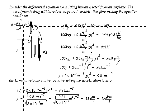
The equation can also be solved using explicit integration, as shown in Figure 1.33 Developing an integral. In this case the equation is separated and rearranged to isolate the ’v’ terms on the left, and time on the right. The term is then integrated in Figure 1.34 Solution of the integral and Figure 1.35 Solution of the integral and application of the initial conditions. The final form of the equation is non-trivial, but contains e-to-t terms, as we would expect. 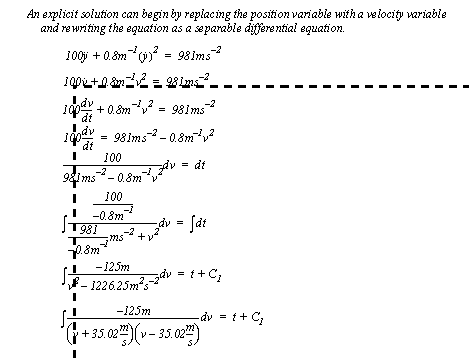
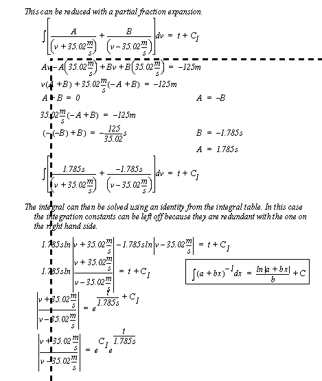
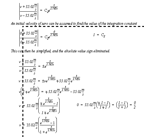
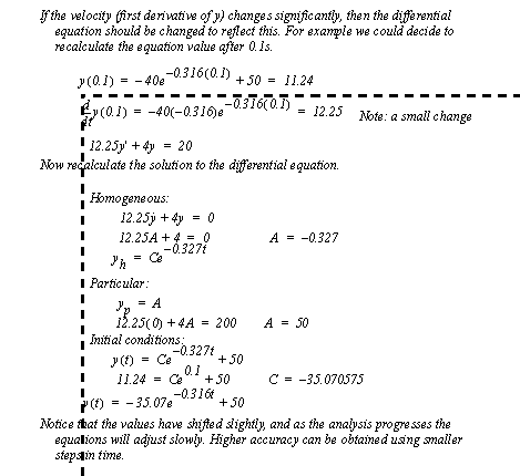
As evident from the example, non-linear equations are involved and don’t utilize routine methods. Typically the numerical methods discussed in the next chapter are preferred. 1.5.2 Non-Linear Equation TermsIf our models include a device that is non-linear and we want to use a linear technique to solve the equation, we will need to linearize the model before we can proceed. A non-linear system can be approximated with a linear equation using the following method. 1. Pick an operating point or range for the component. 2. Find a constant value that relates a change in the input to a change in the output. 4. Use the linear equation for the analysis. A linearized differential equation can be approximately solved using known techniques as long as the system doesn’t travel too far from the linearized point. The example in Figure 1.36 Linearizing a differential equation shows the linearization of a non-linear equation about a given operating point. This equation will be approximately correct as long as the first derivative doesn’t move too far from 100. When this value does, the new velocity can be calculated. 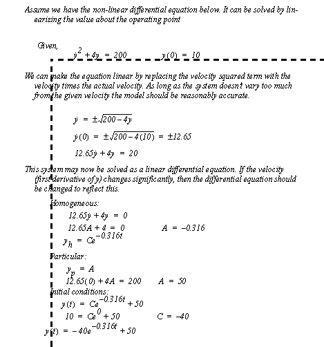
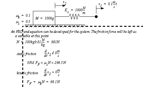
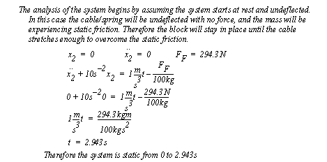
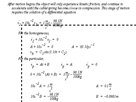
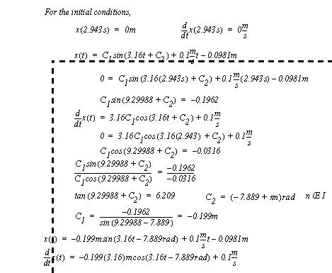
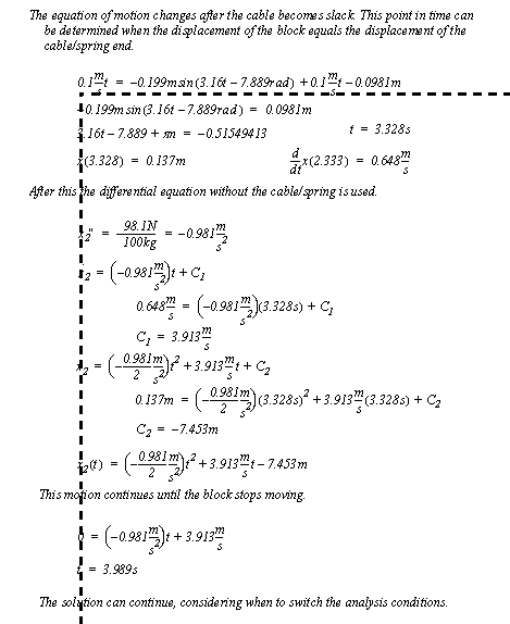
1.5.3 Changing SystemsIn practical systems, the forces at work are continually changing. For example a system often experiences a static friction force when motion is starting, but once motion starts it is replaced with a smaller kinetic friction. Another example is tension in a cable. When in tension a cable acts as a spring. But, when in compression the force goes to zero. Consider the example in Figure 1.38 A differential equation for a mass pulled by a springy cable. A mass is pulled by a springy cable. The right hand side of the cable is being pulled at a constant rate, while the block is free to move, only restricted by friction forces and inertia. At the beginning all components are at rest and undeflected. 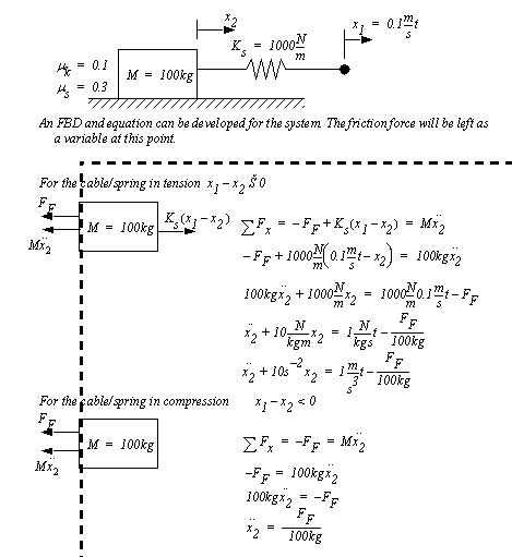
|