10.5 Continuous Distributions
• Histograms are useful for grouped data, but in the cases where the data is continuous, we use distributions of probability.
• In general
- the area under the graph = 1.00000.......
- the graphs often stretch (asymptotically) to infinity
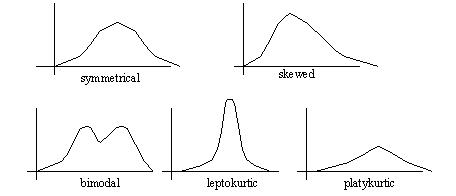
• In specific, some of the distribution properties are,
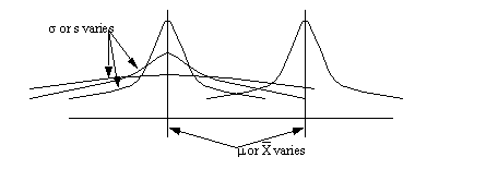
• In addition the centre of the distribution can vary (i.e. the average or mean)
• More on distribution later
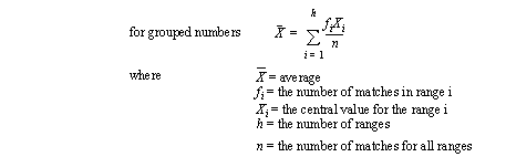
10.5.1 Describing Distribution Centers With Numbers
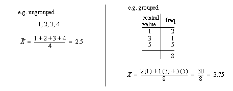
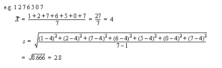
• The best known method is the average. This gives the centre of a distribution
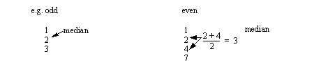
• Another good measure is the median
- If odd number of samples it is the middle number
- if an even number of samples, it is the average of the left and right bounding numbers
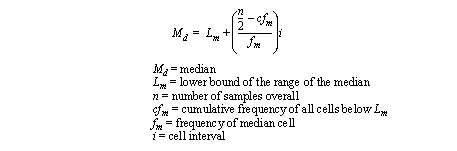
• If the numbers are grouped the median becomes
• Mode can be useful for identifying repeated patterns
- a mode is a repeated value that occurs the most. Multiple modes are possible.
10.5.2 Dispersion As A Measure of Distribution
• The range of values covered by a distribution are important
- Range is the difference between the highest and lowest numbers.
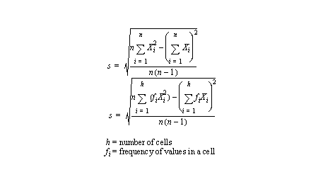
• Standard deviation is a classical measure of grouping (for normal distributions??????????)
- the equation is,
• When we use a standard deviation, we can estimate the distribution of the samples.
• By adding standard deviations to increase the range size, the percentage of samples included are,
• Other formulas for standard deviation are,
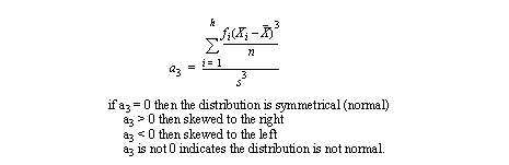
10.5.3 The Shape of the Distribution
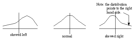
• Skewed functions
• this lack of symmetry tends to indicate a bias in the data (and hence in the real world)
• a skew factor can be calculated
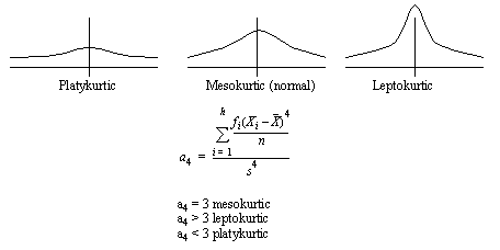
10.5.4 Kurtosis
• This is a peaking in the data
• This is best used for comparison to other values. i.e. you can watch the trends in the values of a4.
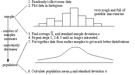
10.5.5 Generalizing From a Few to Many
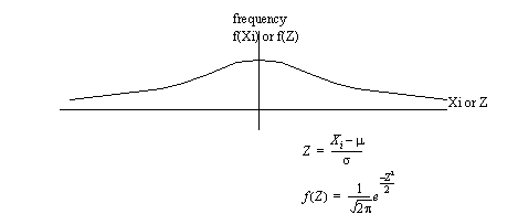
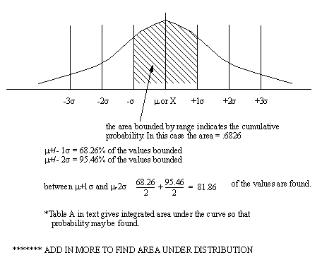
10.5.6 The Normal Curve
• this is a good curve that tends to represent distributions of things in nature (also called Gaussian)
• This distribution can be fitted for populations (μ, σ), or for samples (X, s)
• The area under the curve is 1, and therefore will enclose 100% of the population.
• the parameters vary the shape of the distribution
• The area under the curve indicates the cumulative probability of some event
• When applied to quality ±3σ are used to define a typical “process variability” for the product. This is also known as the upper and lower natural limits (UNL & LNL)
******************* LOOK INTO USE OF SYMBOLS, and UNL, LNL, UCL, LCL, etc.
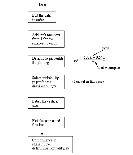
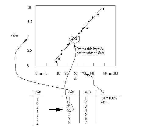
10.5.7 Probability plots
• Procedure